For this Tidy Tuesday challenge we use R to take a look at how voter turnout varies by state for presidential and midterm elections from 1980 to 2014.
library(tidyverse)
library(geofacet)

turnout <- read_csv("https://raw.githubusercontent.com/rfordatascience/tidytuesday/master/data/2018/2018-10-09/voter_turnout.csv") %>%
  select(-X1, -icpsr_state_code, -alphanumeric_state_code)

turnout
# A tibble: 936 x 4
    year state                   votes eligible_voters
   <dbl> <chr>                   <dbl>           <dbl>
 1  2014 United States        83262122       227157964
 2  2014 Alabama               1191274         3588783
 3  2014 Alaska                 285431          520562
 4  2014 Arizona               1537671         4510186
 5  2014 Arkansas               852642         2117881
 6  2014 California            7513972        24440416
 7  2014 Colorado              2080071         3800664
 8  2014 Connecticut           1096556         2577311
 9  2014 Delaware               238110          681526
10  2014 District of Columbia   177176          495899
# … with 926 more rows
Are we missing voting data?
turnout %>%
  summarize(n_missing_votes = sum(is.na(votes)),
            n_missing_eligible_voters = sum(is.na(eligible_voters)))
# A tibble: 1 x 2
   n_missing_votes n_missing_eligible_voters
             <int>                     <int>
 1             223                         0
Yikes, 223 rows in our dataset are missing values for votes. That’s not great. In a more rigorous analysis we would need to get to the bottom of this, but since we are making an exploratory data visualization, we’ll simply make a note of it on the final graphic.
Let’s calculate a few new variables:
- Percent of eligible voters who voted in a given year in each state.
- Percent of eligible voters who voted in a given year in the US.
- Difference between the voter turnout of each state and the national average in a given year.
- Categorical version of differences which will be easier to intepret and will allow us to use a discrete color palette rather than a continuous one.
turnout <- turnout %>%
  select(year, state, votes, eligible_voters) %>%
  filter(!is.na(votes), state %in% c(state.name, "District of Columbia")) %>%  # state.name is a base R constant
  mutate(percent_voted = 100 * votes / eligible_voters) %>%
  group_by(year) %>%
  mutate(national_percent_voted = 100 * sum(votes) / sum(eligible_voters)) %>%
  ungroup() %>%
  mutate(state_vs_national = percent_voted - national_percent_voted,
         state_vs_national_category = cut(state_vs_national,
                                          breaks = c(-Inf, -20, -15, -10, -5, -2, 2, 5, 10, 15, 20, Inf),
                                          ordered_result = TRUE))

turnout
# A tibble: 704 x 6
    year state                percent_voted national_percent_voted state_vs_national state_vs_national_category
   <dbl> <chr>                        <dbl>                  <dbl>             <dbl> <ord>
 1  2014 Alabama                       33.2                   38.3             -5.11 (-10,-5]
 2  2014 Alaska                        54.8                   38.3             16.5  (15,20]
 3  2014 Arizona                       34.1                   38.3             -4.21 (-5,-2]
 4  2014 Arkansas                      40.3                   38.3              1.95 (-2,2]
 5  2014 California                    30.7                   38.3             -7.56 (-10,-5]
 6  2014 Colorado                      54.7                   38.3             16.4  (15,20]
 7  2014 Connecticut                   42.5                   38.3              4.24 (2,5]
 8  2014 Delaware                      34.9                   38.3             -3.37 (-5,-2]
 9  2014 District of Columbia          35.7                   38.3             -2.58 (-5,-2]
10  2014 Florida                       43.3                   38.3              5.01 (5,10]
# … with 694 more rows
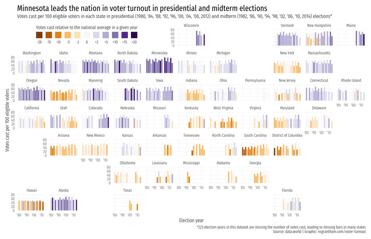
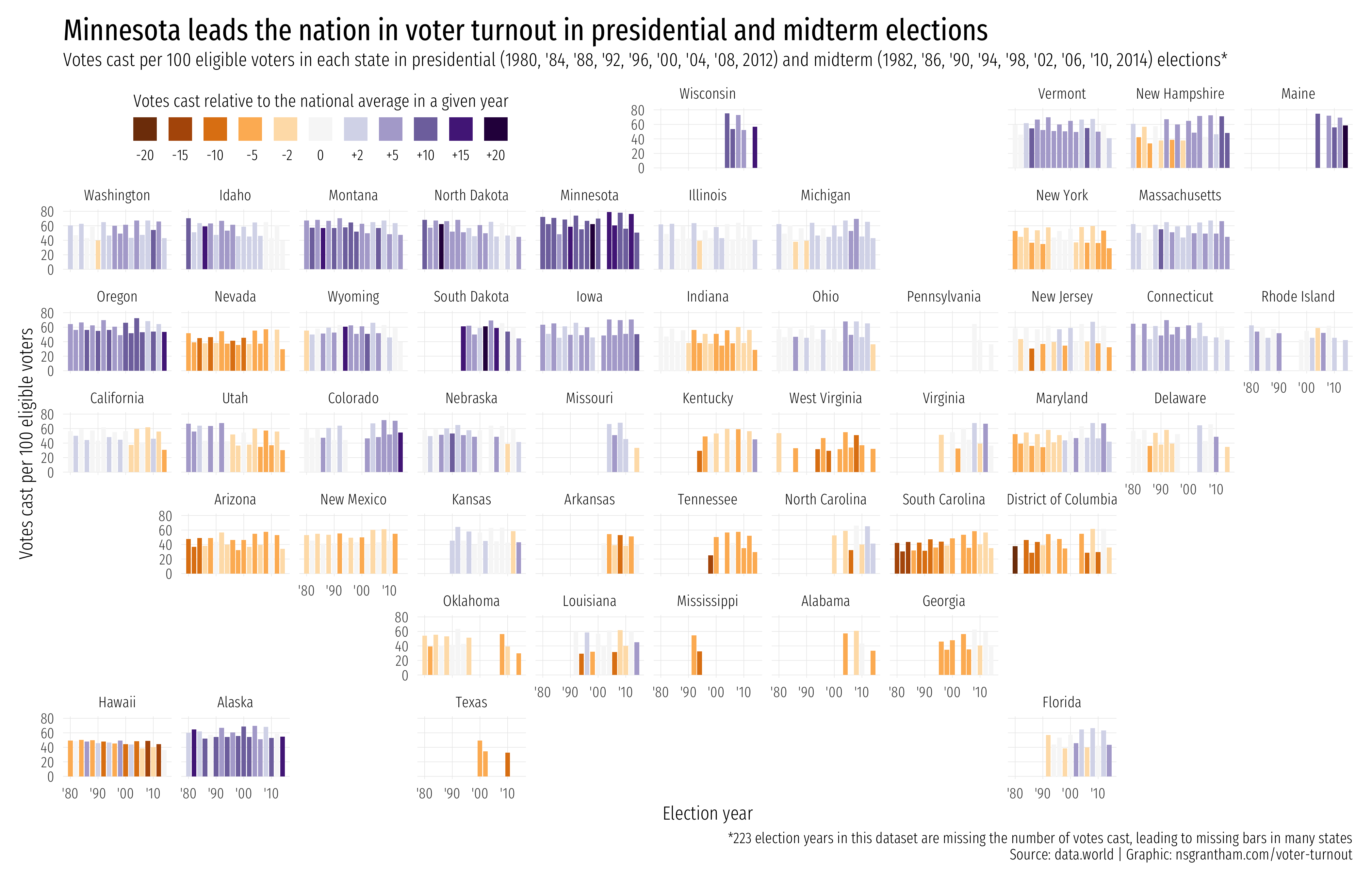
With the data in this form, we can make a bar chart for each state and Washington DC with election year on the x-axis and votes cast per 100 eligible voters on the y-axis.
We’ll use state_vs_national_category to color the bars by the degree to which a state’s voter turnout compares to the national average in a given year.
We’ll alo use facet_geo from the geofacet package to position the state bar charts in the shape of the US.
ggplot(turnout, aes(year, percent_voted, fill = state_vs_national_category)) +
  geom_col(width = 1.7, size = 0) +
  facet_geo(~ state) +
  scale_fill_brewer(labels = c("-20", "-15", "-10", " -5", " -2", " 0 ", " +2", " +5", "+10", "+15", "+20"),
                    type = "div", palette = "PuOr", direction = 1) +
  scale_x_continuous(breaks = c(1980, 1990, 2000, 2010), labels = c("'80", "'90", "'00", "'10")) +
  labs(title = "Minnesota leads the nation in voter turnout in presidential and midterm elections",
       subtitle = "Votes cast per 100 eligible voters in each state in presidential (1980, '84, '88, '92, '96, '00, '04, '08, 2012) and midterm (1982, '86, '90, '94, '98, '02, '06, '10, 2014) elections*",
       caption = "*223 election years in this dataset are missing the number of votes cast, leading to missing bars in many states\nSource: data.world | Graphic: nsgrantham.com/voter-turnout",
       fill = "Votes cast relative to the national average in a given year",
       x = "Election year", y = "Votes cast per 100 eligible voters") +
  guides(fill = guide_legend(title.position = "top", label.position = "bottom", nrow = 1)) +
  theme_minimal(base_family = "Fira Sans Extra Condensed Light", base_size = 14) +
  theme(plot.title = element_text(family = "Fira Sans Extra Condensed", face = "bold", size = 22),
        plot.margin = margin(0.5, 0.5, 0.5, 0.5, "cm"),
        legend.direction = "horizontal",
        legend.position = c(0.2, 0.97),
        legend.spacing.x = unit(0.59, "lines"),
        legend.title = element_text(size = 13),
        panel.grid.major.x = element_line(size = 0.2),
        panel.grid.minor.x = element_blank(),
        panel.grid.major.y = element_line(size = 0.2),
        panel.grid.minor.y = element_blank())

ggsave("voter-turnout.png", width = 14, height = 7)
Nice job Minnesota!