Neal Grantham
Statistical Rethinking homework solutions with Turing.jl
using Distributions  # v0.25
using LinearAlgebra
using ParetoSmooth
using DataFrames     # v1.3
using StatsPlots     # v0.14
using BSplines
using Turing         # v0.19
using CSV            # v0.9

standardize(x) = (x .- mean(x)) ./ std(x);
Homework 1
1. Suppose the globe tossing data (Chapter 2) had turned out to be 4 water and 11 land. Construct the posterior distribution, using grid approximation. Use the same flat prior as in the book.
w = 4;
l = 11;

p_grid = range(0, 1, length=1000);
prior_grid = pdf.(Uniform(0, 1), p_grid);
like_grid = pdf.(Binomial.(w + l, p_grid), w);
post_grid = like_grid .* prior_grid;
post_grid /= sum(post_grid);

plot(p_grid, post_grid, ylab="Density", xlab="p", legend=false)
2. Now suppose the data are 4 water and 2 land. Compute the posterior again, but this time use a prior that is zero below p = 0.5 and a constant above p = 0.5. This corresponds to prior information that a majority of the Earth’s surface is water.
w = 4;
l = 2;

prior_grid = pdf.(Uniform(0.5, 1.), p_grid);
like_grid = pdf.(Binomial.(w + l, p_grid), w);
post_grid = like_grid .* prior_grid;
post_grid /= sum(post_grid);

plot(p_grid, post_grid, ylab="Density", xlab="p", legend=false)
3. For the posterior distribution from 2, compute 89% percentile and HPDI intervals. Compare the widths of these intervals. Which is wider? Why? If you had only the information in the interval, what might you misunderstand about the shape of the posterior distribution?
@model function globetoss(n, w)
    p ~ Uniform(0.5, 1.)
    w ~ Binomial(n, p)
end;

post = sample(globetoss(w + l, w), MH(), 10_000);

quantile(post, q=[0.055, 0.945])
## Quantiles
##   parameters      5.5%     94.5%
##       Symbol   Float64   Float64
##
##            p    0.5243    0.8790
hpd(post, alpha=0.11)
## HPD
##   parameters     lower     upper
##       Symbol   Float64   Float64
##
##            p    0.5002    0.8427
The 89% percentile interval is wider than the 89% HPD interval because the 89% HPD interval is, by definition, the narrowest region with 89% of the posterior probability. If we only had information in the interval, we might completely miss the fact that the distribution is truncated on 0.5 to 1.0!
OPTIONAL CHALLENGE. Suppose there is bias in sampling so that Land is more likely than Water to be recorded. Specifically, assume that 1-in-5 (20%) of Water samples are accidentally recorded instead as Land. First, write a generative simulation of this sampling process. Assuming the true proportion of Water is 0.70, what proportion does your simulation tend to produce instead? Second, using a simulated sample of 20 tosses, compute the unbiased posterior distribution of the true proportion of Water.
If the true proportion of Water is 0.7, and the proportion of Water samples that are accurately recorded as Water is 0.8, then we expect the simulation to tend to produce a proportion of Water of 0.7 * 0.8 = 0.56.
BiasedBinomial(n, p) = Binomial(n, 0.8p);

@model function globetoss(n, w)
    p ~ Uniform(0, 1)
    w ~ BiasedBinomial(n, p)
end;

n = 20;
w = 11;

post = sample(globetoss(n, w), MH(), 10_000)
## Chains MCMC chain (10000×2×1 Array{Float64, 3}):
##
## Iterations        = 1:1:10000
## Number of chains  = 1
## Samples per chain = 10000
## Wall duration     = 0.32 seconds
## Compute duration  = 0.32 seconds
## parameters        = p
## internals         = lp
##
## Summary Statistics
##   parameters      mean       std   naive_se      mcse         ess      rhat    ⋯
##       Symbol   Float64   Float64    Float64   Float64     Float64   Float64    ⋯
##
##            p    0.6804    0.1284     0.0013    0.0022   3381.0880    1.0003    ⋯
##                                                                 1 column omitted
##
## Quantiles
##   parameters      2.5%     25.0%     50.0%     75.0%     97.5%
##       Symbol   Float64   Float64   Float64   Float64   Float64
##
##            p    0.4259    0.5913    0.6838    0.7695    0.9247
density(post)
Notice that the posterior distribution is unbiased. Despite recording 11 Water out of 20 tosses (55% Water), the posterior distribution is concentrated around 0.7, the true proportion of Water.
Homework 2
1. Construct a linear regression of weight as predicted by height, using the adults (age 18 or greater) from the Howell1 dataset. The heights listed below were recorded in the !Kung census, but weights were not recorded for these individuals. Provide predicted weights and 89% compatibility intervals for each of these individuals. That is, fill in the table below, using model-based predictions.
| i | height | expected weight | 89% interval |
|---|---|---|---|
| 1 | 140 | ||
| 2 | 160 | ||
| 3 | 175 |
howell = CSV.read(
    download("https://raw.githubusercontent.com/rmcelreath/rethinking/master/data/Howell1.csv"),
    DataFrame,
    delim=';'
)
## 544×4 DataFrame
##  Row │ height   weight    age      male
##      │ Float64  Float64   Float64  Int64
## ─────┼───────────────────────────────────
##    1 │ 151.765  47.8256      63.0      1
##    2 │ 139.7    36.4858      63.0      0
##    3 │ 136.525  31.8648      65.0      0
##    4 │ 156.845  53.0419      41.0      1
##    5 │ 145.415  41.2769      51.0      0
##    6 │ 163.83   62.9926      35.0      1
##    7 │ 149.225  38.2435      32.0      0
##    8 │ 168.91   55.48        27.0      1
##   ⋮  │    ⋮        ⋮         ⋮       ⋮
##  538 │ 142.875  34.2462      31.0      0
##  539 │  76.835   8.02291      1.0      1
##  540 │ 145.415  31.1278      17.0      1
##  541 │ 162.56   52.1631      31.0      1
##  542 │ 156.21   54.0625      21.0      0
##  543 │  71.12    8.05126      0.0      1
##  544 │ 158.75   52.5316      68.0      1
##                          529 rows omitted
adult = howell[howell.age .>= 18, :];
plot(adult.height, adult.weight, ylab="Adult Weight (kg)", xlab="Adult Height (cm)", seriestype=:scatter, legend=false)
@model function adult_stature(w, h, h̄)
    α ~ Normal(50, 10)
    β ~ LogNormal(0, 1)
    σ ~ Exponential(1)
    μ = α .+ β .* (h .- h̄)
    w ~ MvNormal(μ, σ)
end;

model = adult_stature(adult.weight, adult.height, mean(adult.height));
post = sample(model, NUTS(), 10_000);
preds = predict(adult_stature(missing, [140, 160, 175], mean(adult.height)), post);

mean(preds)  # expected weights
## Mean
##   parameters      mean
##       Symbol   Float64
##
##         w[1]   35.8370
##         w[2]   48.3595
##         w[3]   57.7743
quantile(preds, q=[0.055, 0.945]) # 89% intervals
## Quantiles
##   parameters      5.5%     94.5%
##       Symbol   Float64   Float64
##
##         w[1]   29.2081   42.6792
##         w[2]   41.5726   55.0810
##         w[3]   50.9816   64.6083
2. From the Howell1 dataset, consider only the people younger than 13 years old. Estimate the causal association between age and weight. Assume that age influences weight through two paths. First, age influences height, and height influences weight. Second, age directly influences weight through age-related changes in muscle growth and body proportions. All of this implies this causal model (DAG):

Use a linear regression to estimate the total (not just direct) causal effect of each year of growth on weight. Be sure to carefully consider the priors. Try using prior predictive simulation to assess what they imply.
@model function child_stature(w, a)
    α ~ Normal(4, 1)
    β ~ LogNormal(0, 0.5)
    σ ~ Exponential(0.5)
    μ = α .+ β .* a
    w ~ MvNormal(μ, σ)
end;

child = howell[howell.age .< 13, :];
We assess our priors with prior predictive simulations.
model = child_stature(child.weight, child.age);
prior = sample(model, Prior(), 1_000);
age_seq = collect(0:12);
prior_preds = predict(child_stature(missing, age_seq), prior);
prior_preds = dropdims(prior_preds.value, dims=3)';
plot(repeat(age_seq, size(prior_preds, 2)), vec(prior_preds), ylab="Child Weight (kg)", xlab="Child Age", title="Prior Predictive Simulations", alpha=0.1, seriestype=:scatter, legend=false)
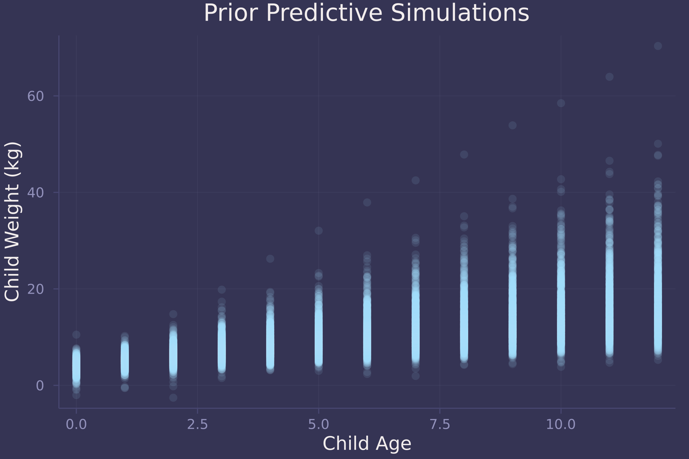
The simulations appear to represent plausible relationships between child age and weight.
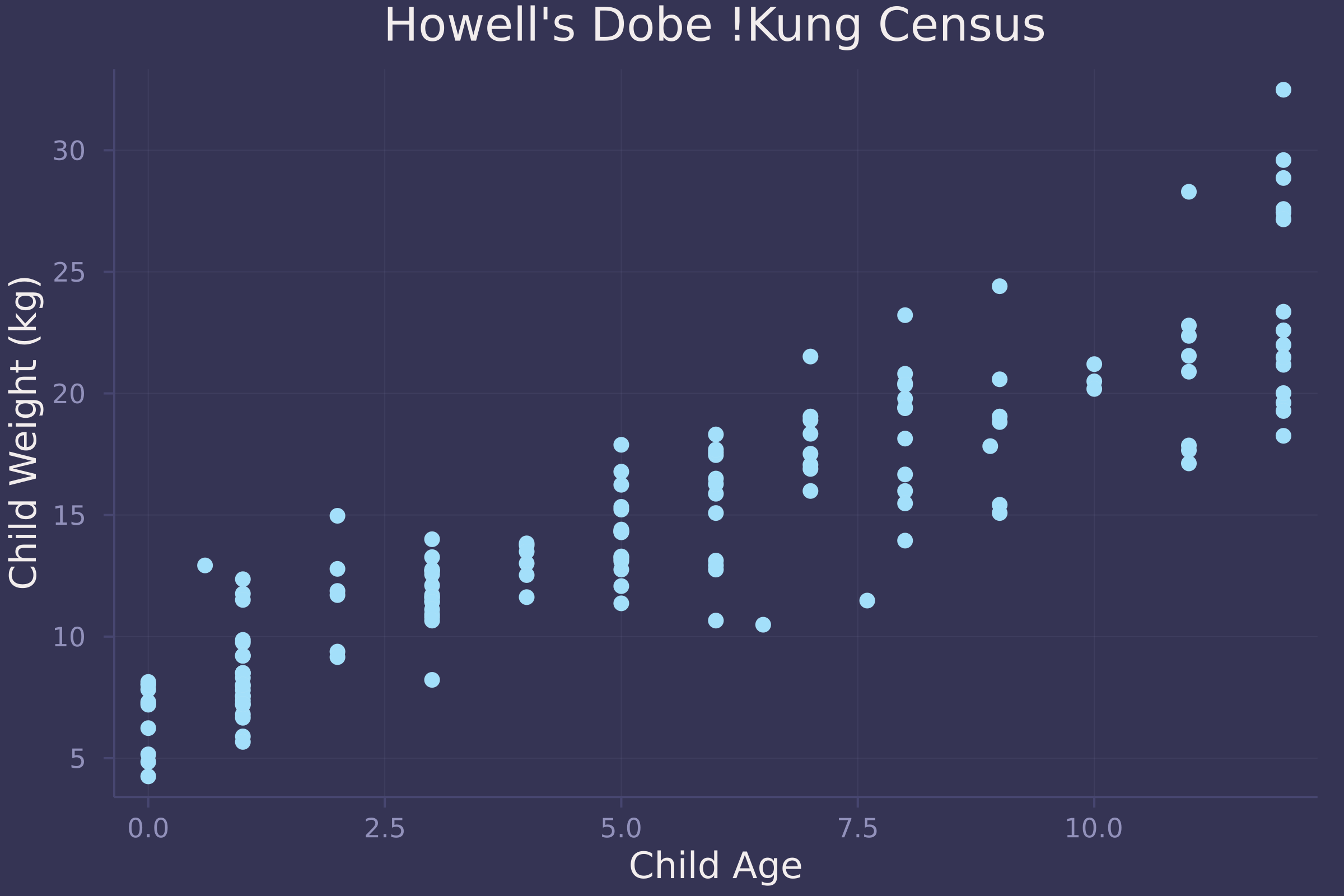
What does the data look like?
plot(child.age, child.weight, ylab="Child Weight (kg)", xlab="Child Age", title="Howell's Dobe !Kung Census", seriestype=:scatter, legend=false)
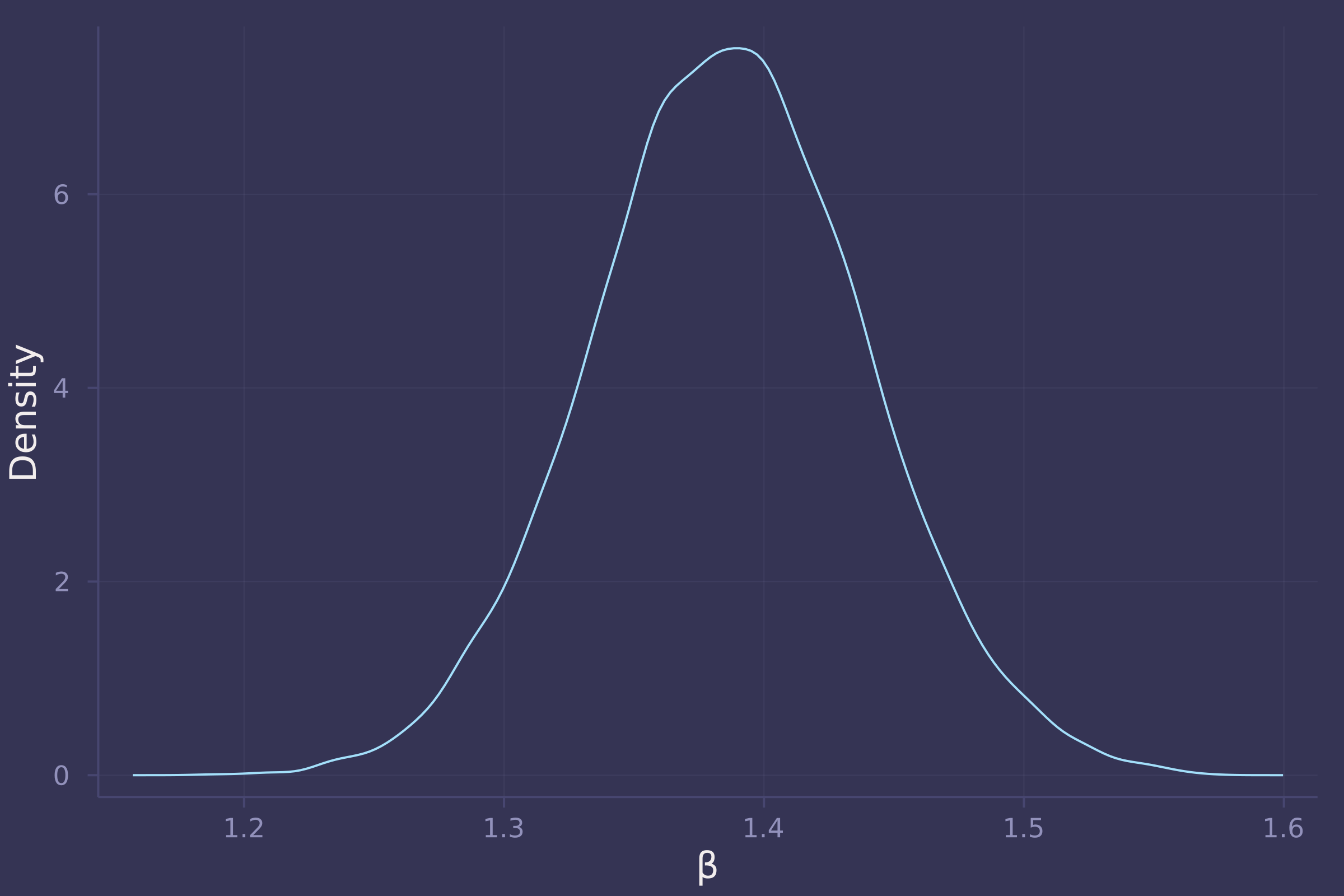
Now we fit a linear regression model to the data and plot the marginal posterior distribution of β, which represents the effect of each year of growth on child weight.
post = sample(model, NUTS(), 10_000)
## Chains MCMC chain (10000×15×1 Array{Float64, 3}):
##
## Iterations        = 1001:1:11000
## Number of chains  = 1
## Samples per chain = 10000
## Wall duration     = 2.73 seconds
## Compute duration  = 2.73 seconds
## parameters        = α, β, σ
## internals         = lp, n_steps, is_accept, acceptance_rate, log_density, hamiltonian_energy, hamiltonian_energy_error, max_hamiltonian_energy_error, tree_depth, numerical_error, step_size, nom_step_size
##
## Summary Statistics
##   parameters      mean       std   naive_se      mcse         ess      rhat    ⋯
##       Symbol   Float64   Float64    Float64   Float64     Float64   Float64    ⋯
##
##            α    7.0735    0.3389     0.0034    0.0047   4914.6959    1.0001    ⋯
##            β    1.3865    0.0528     0.0005    0.0007   5077.9655    1.0000    ⋯
##            σ    2.5251    0.1436     0.0014    0.0019   6465.1057    0.9999    ⋯
##                                                                 1 column omitted
##
## Quantiles
##   parameters      2.5%     25.0%     50.0%     75.0%     97.5%
##       Symbol   Float64   Float64   Float64   Float64   Float64
##
##            α    6.4042    6.8446    7.0713    7.3010    7.7484
##            β    1.2837    1.3518    1.3863    1.4217    1.4927
##            σ    2.2570    2.4268    2.5194    2.6178    2.8275
density(post["β"], ylab="Density", xlab="β", legend=false)
3. Now suppose the causal association between age and weight might be different for boys and girls. Use a single linear regression, with a categorical variable for sex, to estimate the total causal effect of age on weight separately for boys and girls. How do girls and boys differ? Provide one or more posterior contrasts as a summary.
@model function child_stature(w, a, s)
    α ~ filldist(Normal(4, 1), 2)
    β ~ filldist(LogNormal(0, 0.5), 2)
    σ ~ Exponential(0.5)
    μ = α[s] .+ β[s] .* a
    w ~ MvNormal(μ, σ)
end;

model = child_stature(child.weight, child.age, child.male .+ 1);
post = sample(model, NUTS(), 10_000)
## Chains MCMC chain (10000×17×1 Array{Float64, 3}):
##
## Iterations        = 1001:1:11000
## Number of chains  = 1
## Samples per chain = 10000
## Wall duration     = 5.19 seconds
## Compute duration  = 5.19 seconds
## parameters        = α[1], α[2], β[1], β[2], σ
## internals         = lp, n_steps, is_accept, acceptance_rate, log_density, hamiltonian_energy, hamiltonian_energy_error, max_hamiltonian_energy_error, tree_depth, numerical_error, step_size, nom_step_size
##
## Summary Statistics
##   parameters      mean       std   naive_se      mcse         ess      rhat    ⋯
##       Symbol   Float64   Float64    Float64   Float64     Float64   Float64    ⋯
##
##         α[1]    6.5110    0.4451     0.0045    0.0047   6904.7900    1.0000    ⋯
##         α[2]    7.1157    0.4634     0.0046    0.0053   6351.7104    1.0001    ⋯
##         β[1]    1.3552    0.0705     0.0007    0.0007   7058.9105    0.9999    ⋯
##         β[2]    1.4798    0.0721     0.0007    0.0008   6497.3970    1.0004    ⋯
##            σ    2.4642    0.1460     0.0015    0.0016   7756.6571    1.0000    ⋯
##                                                                 1 column omitted
##
## Quantiles
##   parameters      2.5%     25.0%     50.0%     75.0%     97.5%
##       Symbol   Float64   Float64   Float64   Float64   Float64
##
##         α[1]    5.6317    6.2189    6.5110    6.8026    7.3883
##         α[2]    6.1999    6.7999    7.1251    7.4348    8.0154
##         β[1]    1.2166    1.3083    1.3554    1.4020    1.4965
##         β[2]    1.3403    1.4305    1.4782    1.5287    1.6224
##            σ    2.1978    2.3646    2.4593    2.5545    2.7703
age_seq = range(0, 12, length=50);
w_f = predict(child_stature(missing, age_seq, 1), post);
w_m = predict(child_stature(missing, age_seq, 2), post);
w_diff = dropdims(w_m.value .- w_f.value, dims=3)';
w_diff_mean = vec(mean(w_diff, dims=2));
w_diff_50 = mapslices(x -> quantile(x, [0.25, 0.75]), w_diff, dims=2);
w_diff_70 = mapslices(x -> quantile(x, [0.15, 0.85]), w_diff, dims=2);
w_diff_90 = mapslices(x -> quantile(x, [0.05, 0.95]), w_diff, dims=2);
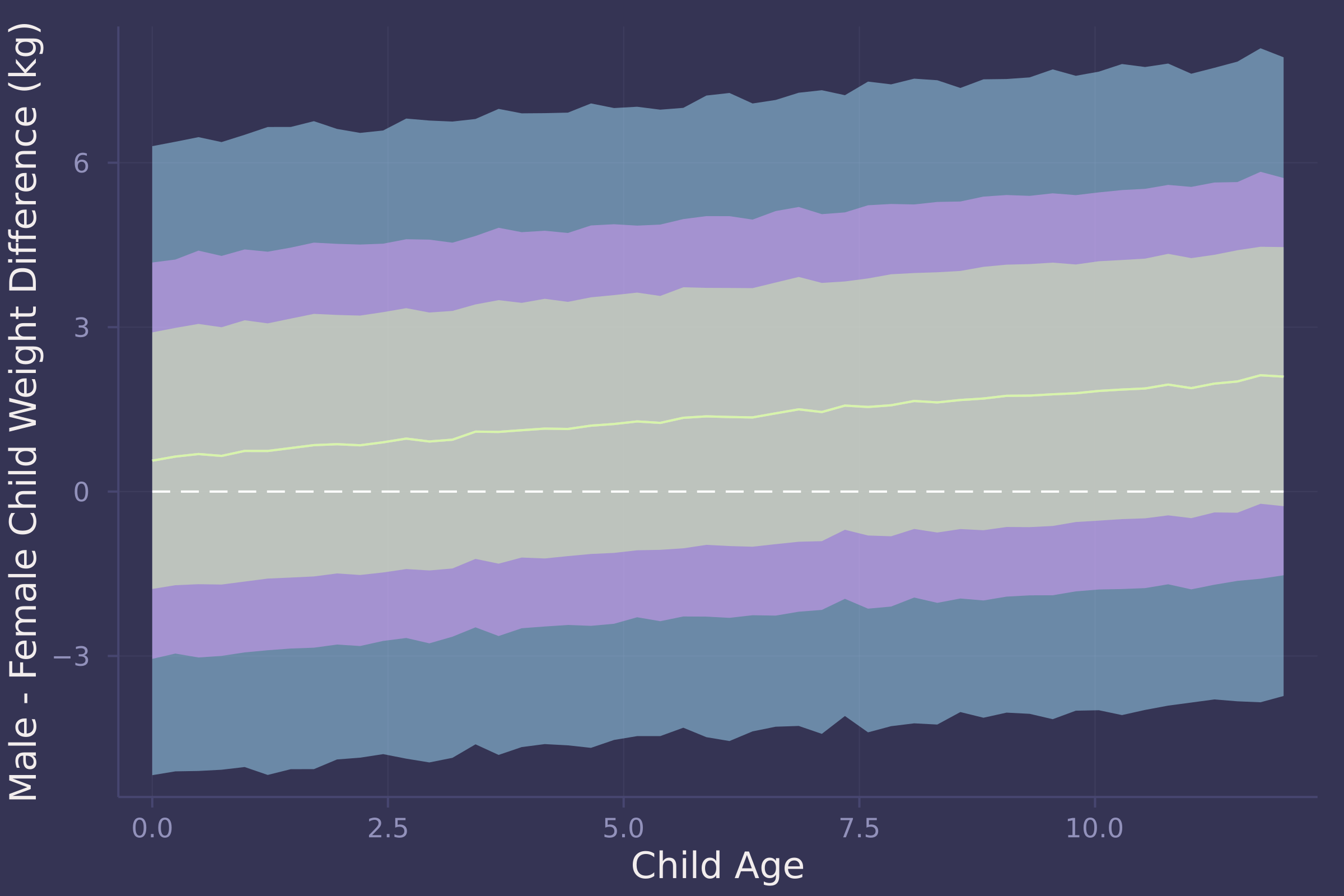
plot(age_seq, w_diff_mean, ribbon=abs.(w_diff_mean .- w_diff_90), ylab="Male - Female Child Weight Difference (kg)", xlab="Child Age");
plot!(age_seq, w_diff_mean, ribbon=abs.(w_diff_mean .- w_diff_70), legend=false);
plot!(age_seq, w_diff_mean, ribbon=abs.(w_diff_mean .- w_diff_50), legend=false);
plot!(age_seq, fill(0, length(age_seq)), line=:dash, color=:white, legend=false)
4. OPTIONAL CHALLENGE. The data in oxboys are growth records for 26 boys measured over 9 periods. I want you to model their growth. Specifically, model the increments in growth from one period (Occasion in the data table) to the next. Each increment is simply the difference between height in one occasion and height in the previous occasion. Since none of these boys shrunk during the study, all of the growth increments are greater than zero. Estimate the posterior distribution of these increments. Constrain the distribution so it is always positive — it should not be possible for the model to think that boys can shrink from year to year. Finally compute the posterior distribution of the total growth over all 9 occasions.
oxboys = CSV.read(
    download("https://raw.githubusercontent.com/rmcelreath/rethinking/master/data/Oxboys.csv"),
    DataFrame,
    delim=';'
);
oxboys = combine(groupby(oxboys, :Subject), :height => diff => :diff);
oxboys = transform(groupby(oxboys, :Subject), :Subject => (x -> 1:length(x)) => :time)
## 208×3 DataFrame
##  Row │ Subject  diff     time
##      │ Int64    Float64  Int64
## ─────┼─────────────────────────
##    1 │       1      2.9      1
##    2 │       1      1.4      2
##    3 │       1      2.3      3
##    4 │       1      0.6      4
##    5 │       1      2.5      5
##    6 │       1      1.5      6
##    7 │       1      1.6      7
##    8 │       1      2.5      8
##   ⋮  │    ⋮        ⋮       ⋮
##  202 │      26      0.8      2
##  203 │      26      1.6      3
##  204 │      26      1.7      4
##  205 │      26      0.5      5
##  206 │      26      2.9      6
##  207 │      26      0.8      7
##  208 │      26      0.5      8
##                193 rows omitted
@model function oxboy_growth(d, t)
    μ ~ filldist(Normal(0, 0.2), length(unique(t)))
    σ ~ Exponential(0.2)
    d ~ MvLogNormal(μ[t], σ)
end;

prior = sample(oxboy_growth(oxboys.diff, oxboys.time), Prior(), 1_000);
prior_preds = predict(oxboy_growth(missing, 1:8), prior);
prior_preds = dropdims(prior_preds.value, dims=3)';
plot(repeat(1:8, size(prior_preds, 2)), vec(prior_preds), ylab="Height increment (cm)", xlab="Time", title="Prior Predictive Simulations", alpha=0.1, seriestype=:scatter, legend=false)
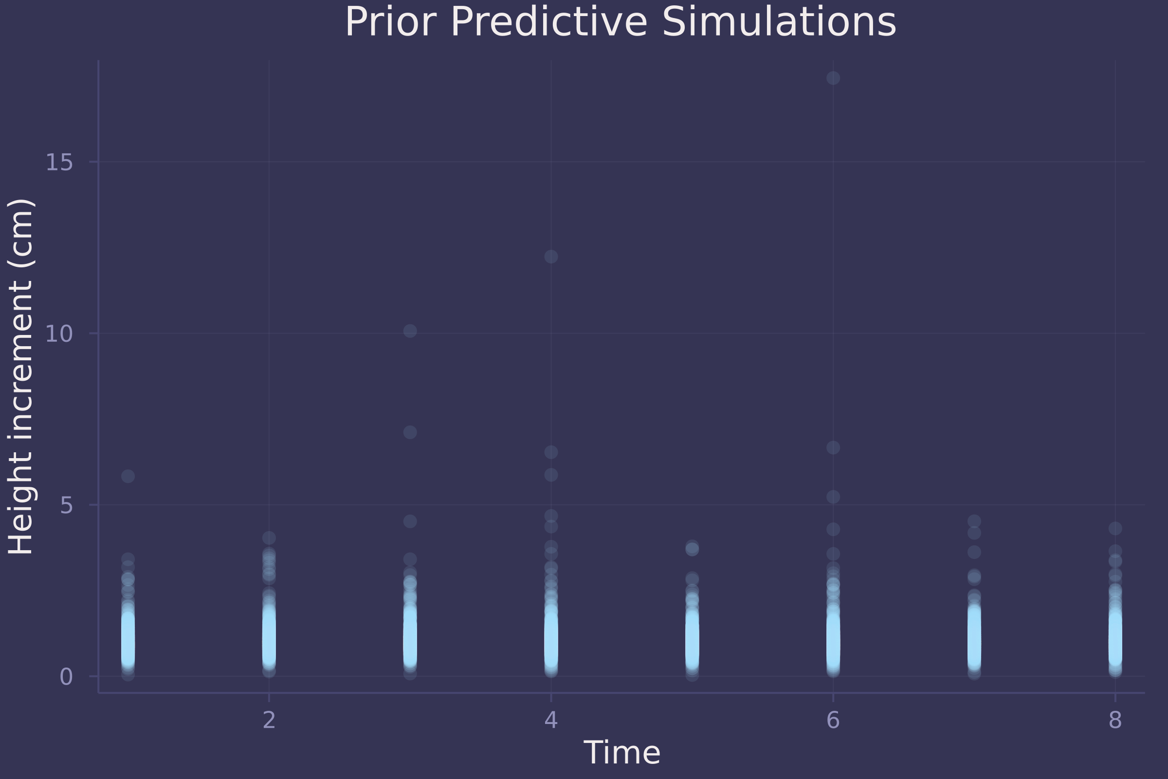
Not great prior predictive simulations. A downside to using the Log-Normal distribution here is that it produces skewed, unrealistically high height increments.
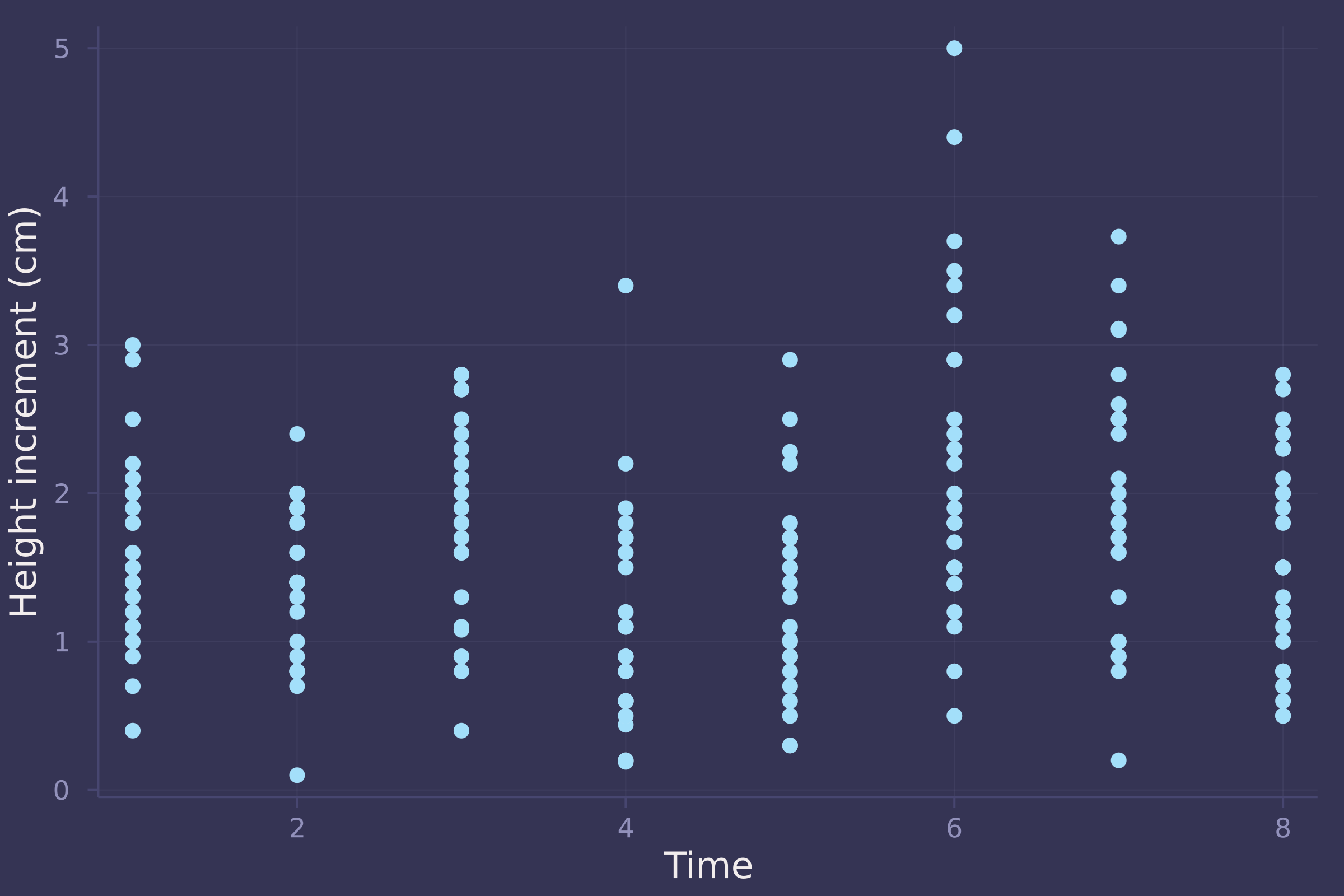
Let’s take a look at the actual data.
plot(oxboys.time, oxboys.diff, ylab="Height increment (cm)", xlab="Time", seriestype=:scatter, legend=false)
model = oxboy_growth(oxboys.diff, oxboys.time);
post = sample(model, MH(), 10_000)
## Chains MCMC chain (10000×10×1 Array{Float64, 3}):
##
## Iterations        = 1:1:10000
## Number of chains  = 1
## Samples per chain = 10000
## Wall duration     = 1.27 seconds
## Compute duration  = 1.27 seconds
## parameters        = μ[1], μ[2], μ[3], μ[4], μ[5], μ[6], μ[7], μ[8], σ
## internals         = lp
##
## Summary Statistics
##   parameters      mean       std   naive_se      mcse       ess      rhat   es ⋯
##       Symbol   Float64   Float64    Float64   Float64   Float64   Float64      ⋯
##
##         μ[1]    0.1066    0.0640     0.0006    0.0060   28.6541    1.1949      ⋯
##         μ[2]    0.0383    0.1057     0.0011    0.0103   24.9660    1.0002      ⋯
##         μ[3]    0.3841    0.1318     0.0013    0.0129   25.4927    1.1567      ⋯
##         μ[4]    0.0904    0.1118     0.0011    0.0108   26.1662    1.0012      ⋯
##         μ[5]   -0.0287    0.1563     0.0016    0.0153   21.6931    2.3444      ⋯
##         μ[6]    0.3885    0.1773     0.0018    0.0176   22.2689    1.7977      ⋯
##         μ[7]    0.1270    0.1957     0.0020    0.0192   21.8922    2.1461      ⋯
##         μ[8]    0.0392    0.1565     0.0016    0.0149   26.0338    1.2843      ⋯
##            σ    0.6287    0.0303     0.0003    0.0028   34.1437    1.0116      ⋯
##                                                                 1 column omitted
##
## Quantiles
##   parameters      2.5%     25.0%     50.0%     75.0%     97.5%
##       Symbol   Float64   Float64   Float64   Float64   Float64
##
##         μ[1]   -0.0525    0.0540    0.1406    0.1406    0.2141
##         μ[2]   -0.1046   -0.0178    0.0321    0.0321    0.3453
##         μ[3]   -0.0298    0.3492    0.3760    0.4851    0.4851
##         μ[4]   -0.1932    0.1032    0.1032    0.1926    0.1926
##         μ[5]   -0.1766   -0.1766   -0.0400    0.0496    0.2723
##         μ[6]   -0.0027    0.2869    0.2869    0.5695    0.5695
##         μ[7]   -0.0537   -0.0537    0.0118    0.3640    0.3982
##         μ[8]   -0.1523   -0.1523    0.1228    0.1228    0.3487
##            σ    0.5276    0.6318    0.6318    0.6446    0.6446
d_sim = predict(oxboy_growth(missing, 1:8), post);
d_sim = dropdims(d_sim.value, dims=3)';
d_mean = vec(mean(d_sim, dims=2));
d_90 = mapslices(x -> quantile(x, [0.05, 0.95]), d_sim, dims=2);
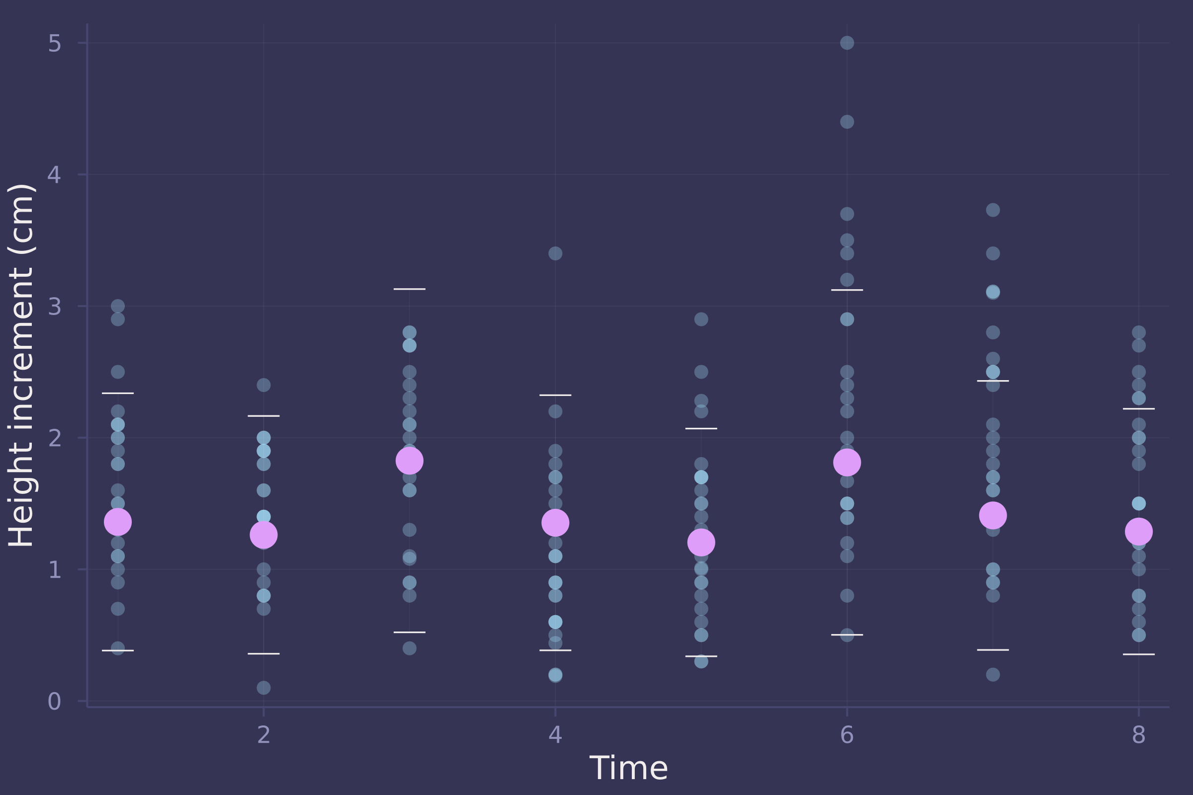
plot(oxboys.time, oxboys.diff, ylab="Height increment (cm)", xlab="Time", seriestype=:scatter, alpha=0.3, legend=false);
plot!(1:8, d_mean, seriestype=:scatter, yerror=(d_mean .- d_90), markersize=8, legend=false)
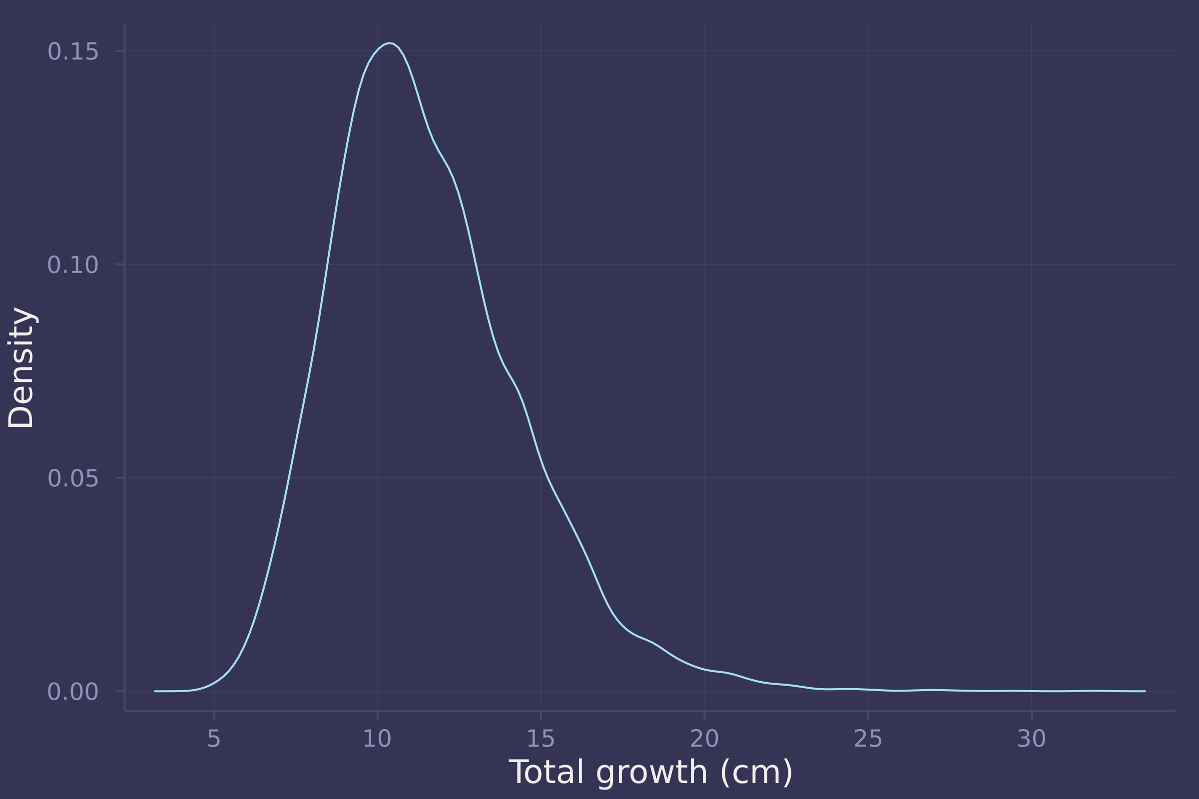
growth_sim = vec(sum(d_sim, dims=1));
density(growth_sim, ylab="Density", xlab="Total growth (cm)", legend=false)
Homework 3
1. The first two problems are based on the same data. The data in foxes are 116 foxes from 30 different urban groups in England. These fox groups are like street gangs. Group size (groupsize) varies from 2 to 8 individuals. Each group maintains its own (almost exclusive) urban territory. Some territories are larger than others. The area variable encodes this information. Some territories also have more avgfood than others. And food influences the weight of each fox. Assume this DAG:

where F is avgfood, G is groupsize, A is area, and W is weight.
Use the backdoor criterion and estimate the total causal influence of A on F . What effect would increasing the area of a territory have on the amount of food inside it?
foxes = CSV.read(
    download("https://raw.githubusercontent.com/rmcelreath/rethinking/master/data/foxes.csv"),
    DataFrame,
    delim=';'
)
## 116×5 DataFrame
##  Row │ group  avgfood  groupsize  area     weight
##      │ Int64  Float64  Int64      Float64  Float64
## ─────┼─────────────────────────────────────────────
##    1 │     1     0.37          2     1.09     5.02
##    2 │     1     0.37          2     1.09     2.84
##    3 │     2     0.53          2     2.05     5.33
##    4 │     2     0.53          2     2.05     6.07
##    5 │     3     0.49          2     2.12     5.85
##    6 │     3     0.49          2     2.12     3.25
##    7 │     4     0.45          2     1.29     4.53
##    8 │     4     0.45          2     1.29     4.09
##   ⋮  │   ⋮       ⋮         ⋮         ⋮        ⋮
##  110 │    29     0.67          4     2.75     5.0
##  111 │    29     0.67          4     2.75     3.81
##  112 │    29     0.67          4     2.75     4.81
##  113 │    29     0.67          4     2.75     3.94
##  114 │    30     0.41          3     1.91     3.16
##  115 │    30     0.41          3     1.91     2.78
##  116 │    30     0.41          3     1.91     3.86
##                                    101 rows omitted
@model function fox_area_on_food_total(f, a)
    α ~ Normal(0, 0.2)
    β ~ Normal(0, 0.5)
    σ ~ Exponential(1)
    μ = α .+ β .* a
    f ~ MvNormal(μ, σ)
end;

standardize(x) = (x .- mean(x)) ./ std(x);

model = fox_area_on_food_total(
    standardize(foxes.avgfood),
    standardize(foxes.area)
);
post = sample(model, NUTS(), 10_000)
## Chains MCMC chain (10000×15×1 Array{Float64, 3}):
##
## Iterations        = 1001:1:11000
## Number of chains  = 1
## Samples per chain = 10000
## Wall duration     = 3.27 seconds
## Compute duration  = 3.27 seconds
## parameters        = α, β, σ
## internals         = lp, n_steps, is_accept, acceptance_rate, log_density, hamiltonian_energy, hamiltonian_energy_error, max_hamiltonian_energy_error, tree_depth, numerical_error, step_size, nom_step_size
##
## Summary Statistics
##   parameters      mean       std   naive_se      mcse          ess      rhat   ⋯
##       Symbol   Float64   Float64    Float64   Float64      Float64   Float64   ⋯
##
##            α   -0.0006    0.0430     0.0004    0.0004   14291.7230    0.9999   ⋯
##            β    0.8762    0.0437     0.0004    0.0004   14647.8061    0.9999   ⋯
##            σ    0.4757    0.0323     0.0003    0.0003   14247.4144    1.0000   ⋯
##                                                                 1 column omitted
##
## Quantiles
##   parameters      2.5%     25.0%     50.0%     75.0%     97.5%
##       Symbol   Float64   Float64   Float64   Float64   Float64
##
##            α   -0.0855   -0.0291   -0.0009    0.0278    0.0844
##            β    0.7889    0.8472    0.8763    0.9053    0.9627
##            σ    0.4172    0.4531    0.4739    0.4964    0.5447
area_seq = range(-2, 2, length=50);
f_preds = predict(fox_area_on_food_total(missing, area_seq), post);
f_preds = dropdims(f_preds.value, dims=3)';

f_preds_mean = vec(mean(f_preds, dims=2));
f_preds_50 = mapslices(x -> quantile(x, [0.25, 0.75]), f_preds, dims=2);
f_preds_70 = mapslices(x -> quantile(x, [0.15, 0.85]), f_preds, dims=2);
f_preds_90 = mapslices(x -> quantile(x, [0.05, 0.95]), f_preds, dims=2);

plot(area_seq, f_preds_mean, ribbon=abs.(f_preds_mean .- f_preds_90), ylab="Average Food (Standardized)", xlab="Area (Standardized)", legend=false);
plot!(area_seq, f_preds_mean, ribbon=abs.(f_preds_mean .- f_preds_70), legend=false);
plot!(area_seq, f_preds_mean, ribbon=abs.(f_preds_mean .- f_preds_50), legend=false)
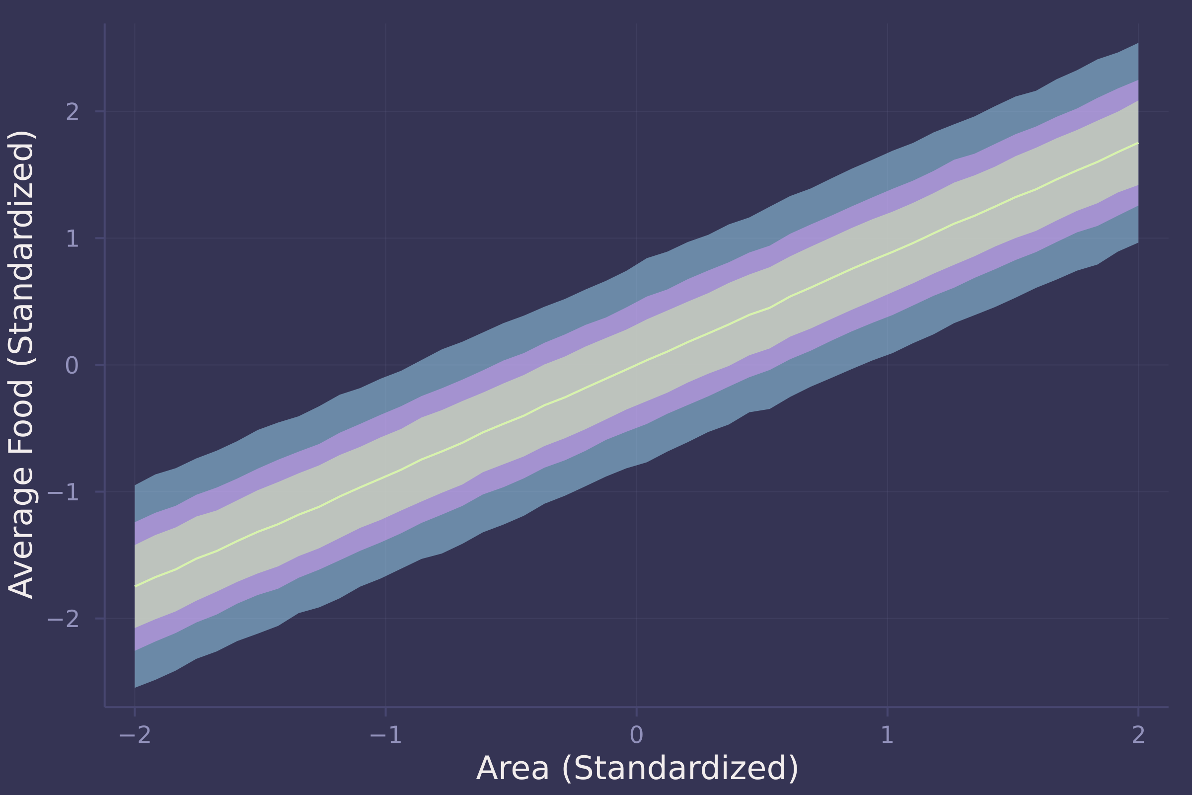
There is a strong positive relationship between area and food — the larger an area, the more food available within it.
2. Now infer both the total and direct causal effects of adding food F to a territory on the weight W of foxes. Which covariates do you need to adjust for in each case? In light of your estimates from this problem and the previous one, what do you think is going on with these foxes? Feel free to speculate — all that matters is that you justify your speculation.
To answer this we will fit two models, one that captures the total causal effect of food on weight, and another that captures the direct causal effect of food on weight.
For the total model, we simply regress weight on food.
@model function fox_food_on_weight_total(w, f)
    α ~ Normal(0, 0.2)
    β ~ Normal(0, 0.5)
    σ ~ Exponential(1)
    μ = α .+ β .* f
    w ~ MvNormal(μ, σ)
end;

model_total = fox_food_on_weight_total(
    standardize(foxes.weight),
    standardize(foxes.avgfood)
);
post_total = sample(model_total, NUTS(), 10_000)
## Chains MCMC chain (10000×15×1 Array{Float64, 3}):
##
## Iterations        = 1001:1:11000
## Number of chains  = 1
## Samples per chain = 10000
## Wall duration     = 2.31 seconds
## Compute duration  = 2.31 seconds
## parameters        = α, β, σ
## internals         = lp, n_steps, is_accept, acceptance_rate, log_density, hamiltonian_energy, hamiltonian_energy_error, max_hamiltonian_energy_error, tree_depth, numerical_error, step_size, nom_step_size
##
## Summary Statistics
##   parameters      mean       std   naive_se      mcse          ess      rhat   ⋯
##       Symbol   Float64   Float64    Float64   Float64      Float64   Float64   ⋯
##
##            α   -0.0014    0.0845     0.0008    0.0007   15177.4868    0.9999   ⋯
##            β   -0.0240    0.0924     0.0009    0.0008   15388.6857    0.9999   ⋯
##            σ    1.0088    0.0659     0.0007    0.0006   14648.4465    0.9999   ⋯
##                                                                 1 column omitted
##
## Quantiles
##   parameters      2.5%     25.0%     50.0%     75.0%     97.5%
##       Symbol   Float64   Float64   Float64   Float64   Float64
##
##            α   -0.1666   -0.0576   -0.0005    0.0551    0.1629
##            β   -0.2055   -0.0861   -0.0244    0.0366    0.1573
##            σ    0.8883    0.9630    1.0060    1.0516    1.1458
density(post_total[:β], ylab="Density", xlab="Parameter Value", label="β")
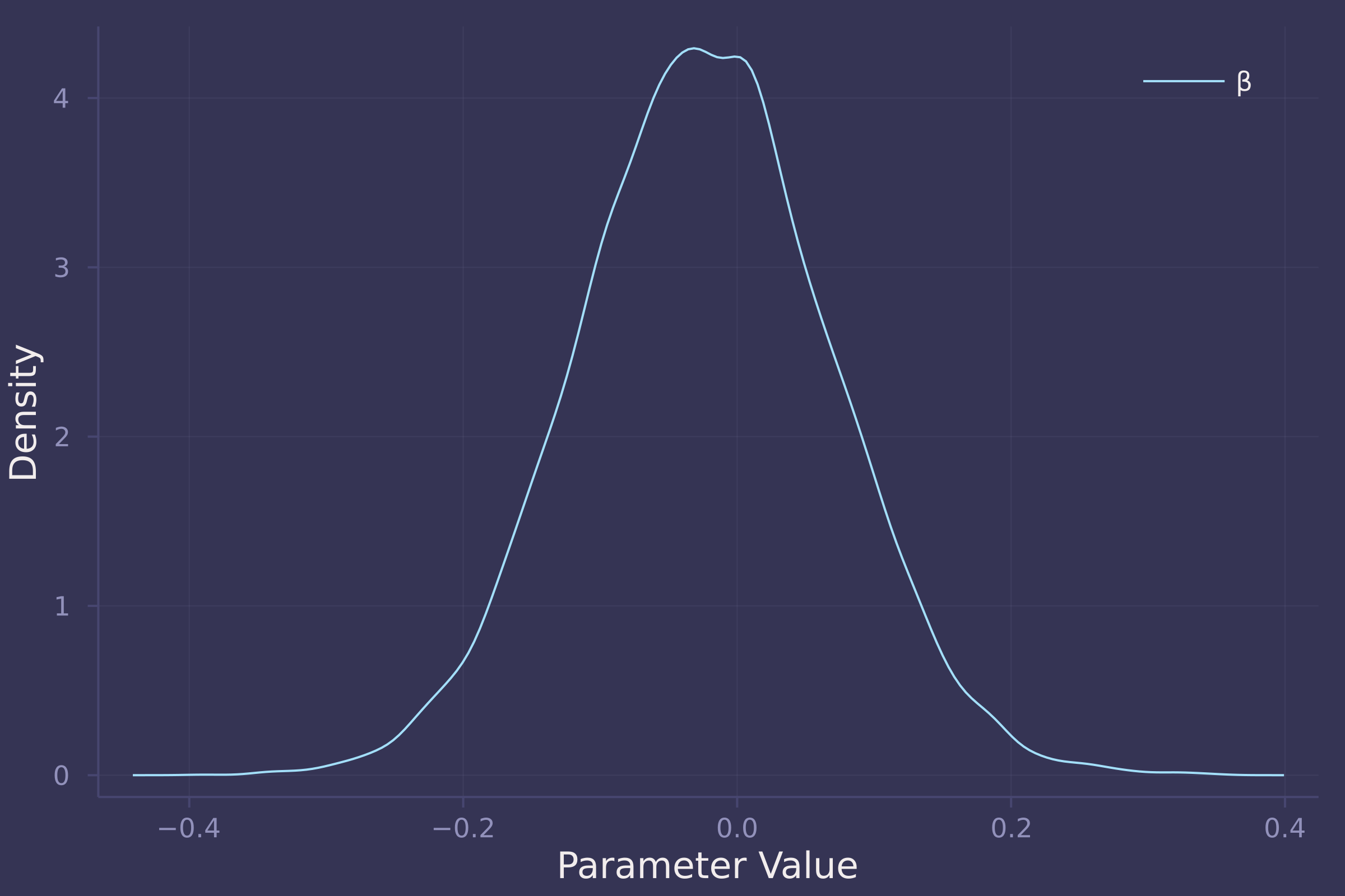
The total effect of food on weight appears negligible. In the total model, β (coefficient of food) is estimated to be approximately centered at zero with an equal spread of both positive and negative values.
Now for the direct model, we regress weight on food and group size, a mediator of food and weight.
@model function fox_food_on_weight_direct(w, f, g)
    α ~ Normal(0, 0.2)
    β ~ Normal(0, 0.5)
    γ ~ Normal(0, 0.5)
    σ ~ Exponential(1)
    μ = α .+ β .* f .+ γ .* g
    w ~ MvNormal(μ, σ)
end;

model_direct = fox_food_on_weight_direct(
    standardize(foxes.weight),
    standardize(foxes.avgfood),
    standardize(foxes.groupsize)
);
post_direct = sample(model_direct, NUTS(), 10_000)
## Chains MCMC chain (10000×16×1 Array{Float64, 3}):
##
## Iterations        = 1001:1:11000
## Number of chains  = 1
## Samples per chain = 10000
## Wall duration     = 4.84 seconds
## Compute duration  = 4.84 seconds
## parameters        = α, β, γ, σ
## internals         = lp, n_steps, is_accept, acceptance_rate, log_density, hamiltonian_energy, hamiltonian_energy_error, max_hamiltonian_energy_error, tree_depth, numerical_error, step_size, nom_step_size
##
## Summary Statistics
##   parameters      mean       std   naive_se      mcse         ess      rhat    ⋯
##       Symbol   Float64   Float64    Float64   Float64     Float64   Float64    ⋯
##
##            α    0.0016    0.0815     0.0008    0.0008   9342.7736    1.0000    ⋯
##            β    0.4727    0.1827     0.0018    0.0022   6287.6286    1.0000    ⋯
##            γ   -0.5682    0.1827     0.0018    0.0022   6440.0546    1.0002    ⋯
##            σ    0.9621    0.0626     0.0006    0.0006   9208.1096    1.0003    ⋯
##                                                                 1 column omitted
##
## Quantiles
##   parameters      2.5%     25.0%     50.0%     75.0%     97.5%
##       Symbol   Float64   Float64   Float64   Float64   Float64
##
##            α   -0.1606   -0.0518    0.0012    0.0546    0.1624
##            β    0.1087    0.3528    0.4728    0.5950    0.8263
##            γ   -0.9222   -0.6931   -0.5714   -0.4460   -0.2011
##            σ    0.8475    0.9178    0.9594    1.0027    1.0924
density([post_direct[:β], post_direct[:γ]], ylab="Density", xlab="Parameter Value", label=["β" "γ"])
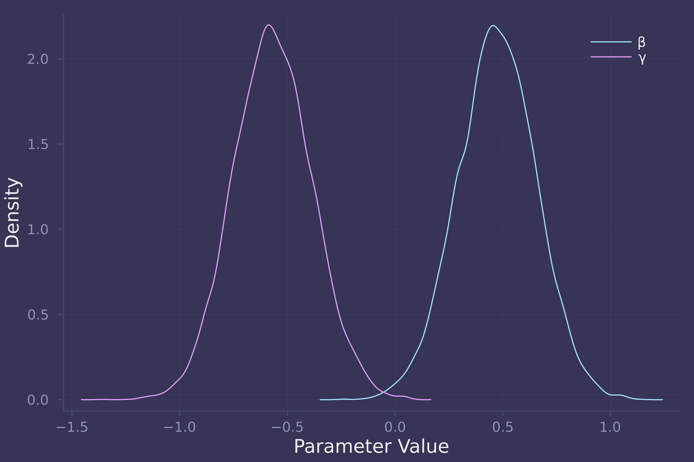
Unlike the total effect, the direct effect of food on weight is reliably positive in a model that also contains group size, which is reliably negative of an almost equal magnitude. In the direct model, β (coefficient of food) is estimated to be centered at 0.5 with most of its density between 0 and 1, while γ (coefficient of group size) is estimated to be centered at -0.6 with most of its density between -1 and 0.
Taken together, the model results suggest that the effect of food on a fox’s weight is almost entirely offset by group size. Put another way, more food available in an urban territory leads to an increase in the number of foxes within that territory, preventing any potential increase in a fox’s weight due to available food.
3. Reconsider the Table 2 Fallacy (from Lecture 6), this time with an unobserved confound U that influences both smoking S and stroke Y . Here’s the modified DAG:

First use the backdoor criterion to determine the adjustment set that allows you to estimate the causal effect of_ X on Y , i.e. P(Y ∣ do(X)) . Second explain the proper interpretation of each coefficient implied by the regression model that corresponds to the adjustment set. Which coefficients (slopes) are causal and which are not? There is not need to fit any models. Just think through the implications.
Alright, no code required for this problem. Let’s think through everything logically.
The backdoor criterion says we need to block any paths that connect X and Y that enter X from the backdoor. There are two such paths.
The first path is X ← A → Y . Here, A is a confounder of X and Y . To block the path, we include A in our adjustment set.
The second path is X ← S → Y . S too is a confounder of X and Y so we also include S in our adjustment set to the block path.
Now, with the adjustment set {A, S} we can properly estimate the causal effect of X on Y . Great! So what’s the problem?
The unobserved variable U wreaks havoc on the other coefficients in the model, contributing to a Table 2 Fallacy.
Take the variable A . As we have conditioned on A and S , and S is a collider of A and U , our estimate of the effect of A on Y in our model is biased by U .
Similarly, U is a confounder of S and Y , biasing the estimate of the effect of S on Y as well.
The takeaway here is that even with an adjustment set that allows us to properly estimate the causal effect of X on Y , we are not guaranteed unbiased estimates of other coefficients in the model which may be polluted by unobserved variables we are unable to control for.
4. OPTIONAL CHALLENGE. Write a synthetic data simulation for the causal model shown in Problem 3. Be sure to include the unobserved confound in the simulation. Choose any functional relationships that you like — you don’t have to get the epidemiology correct. You just need to honor the causal structure. Then design a regression model to estimate the influence of X on Y and use it on your synthetic data. How lrge of a sample do you need to reliably estimate P(Y ∣ do(X)) ? Define “reliably” as you like, but justify your definition.
First, we define a function to generate synthetic data. As the DAG in Problem 3 models the risk of stroke, represented by Y , we call the function generate_strokes() (at the risk of sounding like a diabolical supervillain).
function generate_strokes(n; β = 1)
    a = randn(n)
    u = randn(n)
    s = rand.(Normal.(a .+ u))
    x = rand.(Normal.(a .+ s))
    y = rand.(Normal.(a .+ s .+ u .+ β .* x))
    DataFrame(:x => x, :y => y, :a => a, :s => s)
end;
We’ll also define a regression model called model_strokes().
@model function model_strokes(y, x, a, s)
    α ~ Normal(0, 1)
    β ~ Normal(0, 1)
    γ ~ Normal(0, 1)
    δ ~ Normal(0, 1)
    σ ~ Exponential(1)
    μ = α .+ β .* x .+ γ .* a .+ δ .* s
    y ~ MvNormal(μ, σ)
end;
And finally a simulation function called simulate_strokes() which generates a dataset given a sample size n, fits a model, samples from the posterior, and makes a density plot of β which it adds to an existing base plot p.
function simulate_strokes!(p, n)
    strokes = generate_strokes(n)
    model = model_strokes(strokes.y, strokes.x, strokes.a, strokes.s)
    post = sample(model, NUTS(), 10_000)
    density!(p, post[:β])
end;
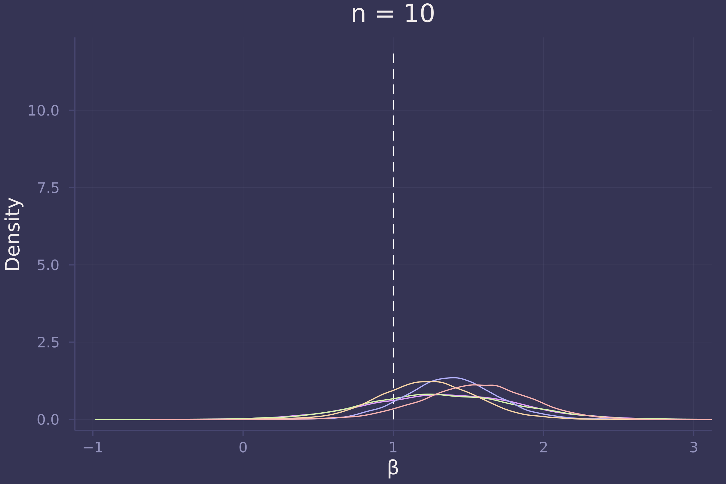
Now let’s investigate the accuracy of our estimate of β under three sample sizes: 10, 100, and 1,000.
using Random
Random.seed!(42);

p = plot([1, 1], [0, 12], ylab="Density", xlab="β", xlims=[-1, 3], line=:dash, color=:white, legend=false);
p10 = deepcopy(p);
p100 = deepcopy(p);
p1000 = deepcopy(p);
for _ in 1:5
    simulate_strokes!(p10, 10);
    simulate_strokes!(p100, 100);
    simulate_strokes!(p1000, 1000);
end;

plot!(p10, title="n = 10")
plot!(p100, title="n = 100")
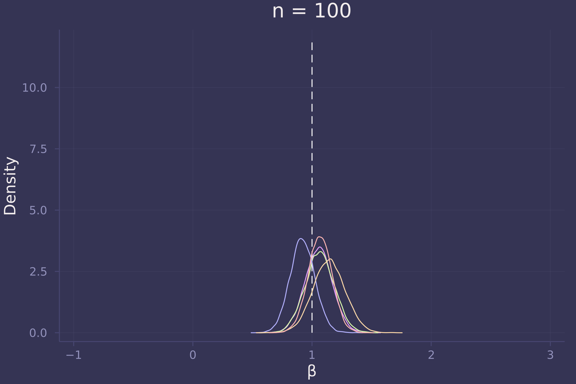
plot!(p1000, title="n = 1000")
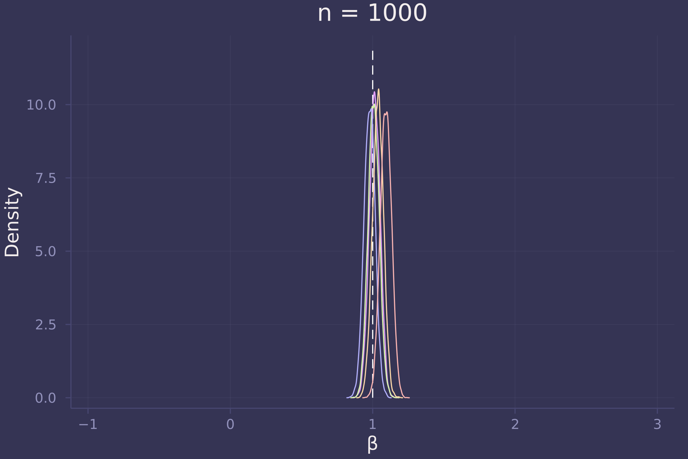
Foregoing a formal definition of “reliable” (as the question insists), it appears as though the estimates of β become reliable-ish with a sample size approaching 100.
Homework 4
1. Revisit the marriage, age, and happiness collider bias example from Chapter 6. Run models m6.9 and m6.10 (pages 178-179). Compare these two models using PSIS and WAIC. Which model is expected to make better predictions, according to these criteria? On the basis of the causal model, how should you interpret the parameter estimates from the model preferred by PSIS and WAIC?
function generate_persons(; n_years=1000, max_age=65, n_births=20, age_of_marriage=18)
    # https://github.com/rmcelreath/rethinking/blob/master/R/sim_happiness.R

    invlogit(x) = 1 ./ (exp(-x) .+ 1)
    age = fill(1, n_births)
    married = fill(false, n_births)
    happiness = collect(range(-2, 2, length=n_births))

    for _ in 1:n_years
        age .+= 1
        append!(age, fill(1, n_births))
        append!(married, fill(false, n_births))
        append!(happiness, collect(range(-2, 2, length=n_births)))

        for i in eachindex(age, married, happiness)
            if age[i] >= age_of_marriage && !married[i]
                married[i] = rand(Bernoulli(invlogit(happiness[i] - 4)))
            end
        end

        deaths = findall(age .> max_age)
        deleteat!(age, deaths)
        deleteat!(married, deaths)
        deleteat!(happiness, deaths)
    end

    DataFrame(
        age = age,
        married = convert.(Int, married),
        happiness = happiness
    )
end;

persons = generate_persons();
adults = persons[persons.age .> 17, :];
min_age, max_age = extrema(adults.age);
adults.age = (adults.age .- min_age) ./ (max_age - min_age);

@model function with_collider(h, a, m)
    α ~ filldist(Normal(0, 1), 2)
    β ~ Normal(0, 2)
    σ ~ Exponential(1)
    μ = α[m] .+ β .* a
    h .~ Normal.(μ, σ)
end;

model_with_collider = with_collider(
    adults.happiness,
    adults.age,
    adults.married .+ 1
);
post_with_collider = sample(model_with_collider, NUTS(), 10_000)
## Chains MCMC chain (10000×16×1 Array{Float64, 3}):
##
## Iterations        = 1001:1:11000
## Number of chains  = 1
## Samples per chain = 10000
## Wall duration     = 16.23 seconds
## Compute duration  = 16.23 seconds
## parameters        = α[1], α[2], β, σ
## internals         = lp, n_steps, is_accept, acceptance_rate, log_density, hamiltonian_energy, hamiltonian_energy_error, max_hamiltonian_energy_error, tree_depth, numerical_error, step_size, nom_step_size
##
## Summary Statistics
##   parameters      mean       std   naive_se      mcse         ess      rhat    ⋯
##       Symbol   Float64   Float64    Float64   Float64     Float64   Float64    ⋯
##
##         α[1]   -0.2066    0.0641     0.0006    0.0009   5215.8579    1.0000    ⋯
##         α[2]    1.2387    0.0879     0.0009    0.0013   4748.6592    1.0003    ⋯
##            β   -0.7526    0.1150     0.0011    0.0017   4351.4088    0.9999    ⋯
##            σ    1.0109    0.0233     0.0002    0.0003   7107.2851    1.0000    ⋯
##                                                                 1 column omitted
##
## Quantiles
##   parameters      2.5%     25.0%     50.0%     75.0%     97.5%
##       Symbol   Float64   Float64   Float64   Float64   Float64
##
##         α[1]   -0.3321   -0.2498   -0.2072   -0.1634   -0.0791
##         α[2]    1.0675    1.1796    1.2387    1.2964    1.4118
##            β   -0.9782   -0.8299   -0.7523   -0.6766   -0.5229
##            σ    0.9662    0.9952    1.0103    1.0261    1.0586
@model function without_collider(h, a)
    α ~ Normal(0, 1)
    β ~ Normal(0, 2)
    σ ~ Exponential(1)
    μ = α .+ β .* a
    h .~ Normal.(μ, σ)
end;

model_without_collider = without_collider(
    adults.happiness,
    adults.age
);
post_without_collider = sample(model_without_collider, NUTS(), 10_000)
## Chains MCMC chain (10000×15×1 Array{Float64, 3}):
##
## Iterations        = 1001:1:11000
## Number of chains  = 1
## Samples per chain = 10000
## Wall duration     = 7.74 seconds
## Compute duration  = 7.74 seconds
## parameters        = α, β, σ
## internals         = lp, n_steps, is_accept, acceptance_rate, log_density, hamiltonian_energy, hamiltonian_energy_error, max_hamiltonian_energy_error, tree_depth, numerical_error, step_size, nom_step_size
##
## Summary Statistics
##   parameters      mean       std   naive_se      mcse         ess      rhat    ⋯
##       Symbol   Float64   Float64    Float64   Float64     Float64   Float64    ⋯
##
##            α   -0.0003    0.0772     0.0008    0.0011   4709.7550    0.9999    ⋯
##            β    0.0004    0.1337     0.0013    0.0020   4485.6562    0.9999    ⋯
##            σ    1.2160    0.0280     0.0003    0.0004   6816.9221    0.9999    ⋯
##                                                                 1 column omitted
##
## Quantiles
##   parameters      2.5%     25.0%     50.0%     75.0%     97.5%
##       Symbol   Float64   Float64   Float64   Float64   Float64
##
##            α   -0.1505   -0.0518    0.0004    0.0510    0.1525
##            β   -0.2633   -0.0914    0.0000    0.0887    0.2645
##            σ    1.1630    1.1968    1.2151    1.2347    1.2731
psis_loo(model_with_collider, post_with_collider, source=:mcmc)
# -1360

psis_loo(model_without_collider, post_without_collider, source=:mcmc)
# -1551
2. Reconsider the urban fox analysis from Homework 3. On the basis of PSIS and WAIC scores, which combination of variables best predicts body weight ( W , weight)? How would you interpret the estimates from the best scoring model?
foxes.area = standardize(foxes.area);
foxes.avgfood = standardize(foxes.avgfood);
foxes.groupsize = standardize(foxes.groupsize);
foxes.weight = standardize(foxes.weight);

@model function fox1(w, x)
    α ~ Normal(0, 0.2)
    β ~ Normal(0, 0.5)
    σ ~ Exponential(1)
    μ = α .+ β .* x
    w .~ Normal.(μ, σ)
end;

@model function fox2(w, x, y)
    α ~ Normal(0, 0.2)
    β ~ Normal(0, 0.5)
    γ ~ Normal(0, 0.5)
    σ ~ Exponential(1)
    μ = α .+ β .* x .+ γ .* y
    w .~ Normal.(μ, σ)
end;

@model function fox3(w, x, y, z)
    α ~ Normal(0, 0.2)
    β ~ Normal(0, 0.5)
    γ ~ Normal(0, 0.5)
    δ ~ Normal(0, 0.5)
    σ ~ Exponential(1)
    μ = α .+ β .* x .+ γ .* y .+ δ .* z
    w .~ Normal.(μ, σ)
end;

model_f = fox1(foxes.weight, foxes.avgfood);
model_g = fox1(foxes.weight, foxes.groupsize);
model_fa = fox2(foxes.weight, foxes.avgfood, foxes.area);
model_fg = fox2(foxes.weight, foxes.avgfood, foxes.groupsize);
model_fga = fox3(foxes.weight, foxes.avgfood, foxes.groupsize, foxes.area);

post_f = sample(model_f, NUTS(), 10_000);
post_g = sample(model_g, NUTS(), 10_000);
post_fa = sample(model_fa, NUTS(), 10_000);
post_fg = sample(model_fg, NUTS(), 10_000);
post_fga = sample(model_fga, NUTS(), 10_000);

psis_loo(model_f, post_f, source=:mcmc)      # -166.60
psis_loo(model_g, post_g, source=:mcmc)      # -165.24
psis_loo(model_fa, post_fa, source=:mcmc)    # -167.17
psis_loo(model_fg, post_fg, source=:mcmc)    # -161.78
psis_loo(model_fga, post_fga, source=:mcmc)  # -161.43
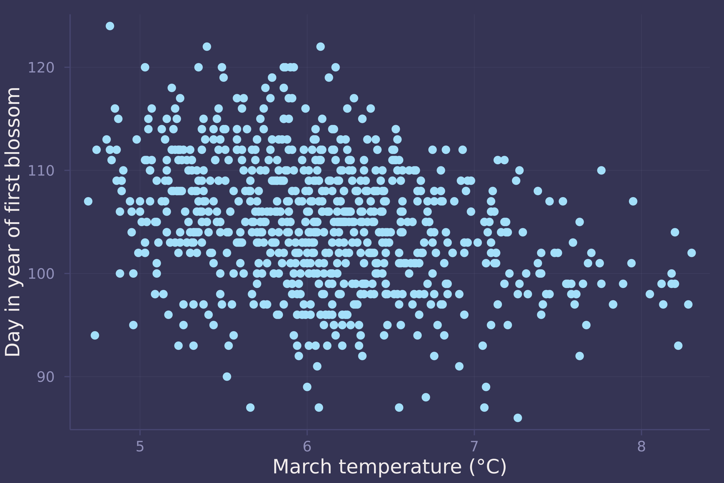
3. Build a predictive model of the relationship show on the cover of the book, the relationship between the timing of cherry blossoms and March temperature in the same year. The data are in cherry_blossoms. Consider at least two functions to predict doy with temp. Compare them with PSIS or WAIC.
Suppose March temperatures reach 9 degrees by the year 2050. What does your best model predict for the predictive distribution of the day-in-year the cherry trees will blossom?
blossoms = CSV.read(
    download("https://raw.githubusercontent.com/rmcelreath/rethinking/master/data/cherry_blossoms.csv"),
    DataFrame,
    delim=';',
    missingstring="NA"
)
## 1215×5 DataFrame
##   Row │ year   doy      temp      temp_upper  temp_lower
##       │ Int64  Int64?   Float64?  Float64?    Float64?
## ──────┼──────────────────────────────────────────────────
##     1 │   801  missing   missing     missing     missing
##     2 │   802  missing   missing     missing     missing
##     3 │   803  missing   missing     missing     missing
##     4 │   804  missing   missing     missing     missing
##     5 │   805  missing   missing     missing     missing
##     6 │   806  missing   missing     missing     missing
##     7 │   807  missing   missing     missing     missing
##     8 │   808  missing   missing     missing     missing
##   ⋮   │   ⋮       ⋮        ⋮          ⋮           ⋮
##  1209 │  2009       95   missing     missing     missing
##  1210 │  2010       95   missing     missing     missing
##  1211 │  2011       99   missing     missing     missing
##  1212 │  2012      101   missing     missing     missing
##  1213 │  2013       93   missing     missing     missing
##  1214 │  2014       94   missing     missing     missing
##  1215 │  2015       93   missing     missing     missing
##                                         1200 rows omitted
dropmissing!(blossoms, [:doy, :temp])
## 787×5 DataFrame
##  Row │ year   doy    temp     temp_upper  temp_lower
##      │ Int64  Int64  Float64  Float64?    Float64?
## ─────┼───────────────────────────────────────────────
##    1 │   851    108     7.38       12.1         2.66
##    2 │   864    100     6.42        8.69        4.14
##    3 │   866    106     6.44        8.11        4.77
##    4 │   889    104     6.83        8.48        5.19
##    5 │   891    109     6.98        8.96        5.0
##    6 │   892    108     7.11        9.11        5.11
##    7 │   894    106     6.98        8.4         5.55
##    8 │   895    104     7.08        8.57        5.58
##   ⋮  │   ⋮      ⋮       ⋮         ⋮           ⋮
##  781 │  1974     99     8.18        8.78        7.58
##  782 │  1975    100     8.18        8.76        7.6
##  783 │  1976     99     8.2         8.77        7.63
##  784 │  1977     93     8.22        8.78        7.66
##  785 │  1978    104     8.2         8.78        7.61
##  786 │  1979     97     8.28        8.83        7.73
##  787 │  1980    102     8.3         8.86        7.74
##                                      772 rows omitted
plot(blossoms.temp, blossoms.doy, ylab="Day in year of first blossom", xlab="March temperature (°C)", seriestype=:scatter, legend=false)
mean_doy = mean(blossoms.doy);
std_doy = std(blossoms.doy);
blossoms.doy = standardize(blossoms.doy);

mean_temp = mean(blossoms.temp);
std_temp = std(blossoms.temp);
blossoms.temp = standardize(blossoms.temp);

@model function blossom_line(d, t)
    α ~ Normal(0, 0.2)
    β ~ Normal(0, 0.5)
    σ ~ Exponential(1)
    μ = α .+ β .* t
    d .~ Normal.(μ, σ)
end;

model_line = blossom_line(blossoms.doy, blossoms.temp);
post_line = sample(model_line, NUTS(), 10_000)
## Chains MCMC chain (10000×15×1 Array{Float64, 3}):
##
## Iterations        = 1001:1:11000
## Number of chains  = 1
## Samples per chain = 10000
## Wall duration     = 4.06 seconds
## Compute duration  = 4.06 seconds
## parameters        = α, β, σ
## internals         = lp, n_steps, is_accept, acceptance_rate, log_density, hamiltonian_energy, hamiltonian_energy_error, max_hamiltonian_energy_error, tree_depth, numerical_error, step_size, nom_step_size
##
## Summary Statistics
##   parameters      mean       std   naive_se      mcse          ess      rhat   ⋯
##       Symbol   Float64   Float64    Float64   Float64      Float64   Float64   ⋯
##
##            α    0.0002    0.0328     0.0003    0.0002   17025.7063    1.0000   ⋯
##            β   -0.3252    0.0341     0.0003    0.0003   12714.6852    1.0001   ⋯
##            σ    0.9464    0.0237     0.0002    0.0002   15815.9987    0.9999   ⋯
##                                                                 1 column omitted
##
## Quantiles
##   parameters      2.5%     25.0%     50.0%     75.0%     97.5%
##       Symbol   Float64   Float64   Float64   Float64   Float64
##
##            α   -0.0650   -0.0213    0.0002    0.0220    0.0646
##            β   -0.3920   -0.3484   -0.3254   -0.3023   -0.2571
##            σ    0.9012    0.9302    0.9460    0.9620    0.9946
@model function blossom_splines(d, B)
    α ~ Normal(0, 0.2)
    β ~ filldist(Normal(0, 0.5), size(B, 2))
    σ ~ Exponential(1)
    μ = α .+ B * β
    @. d ~ Normal(μ, σ)
end;

n_knots = 10;
breakpoints = range(extrema(blossoms.temp)..., length=n_knots);
basis = BSplineBasis(4, breakpoints);
B = basismatrix(basis, blossoms.temp);

model_splines = blossom_splines(blossoms.doy, B);
post_splines = sample(model_splines, NUTS(), 10_000)
## Chains MCMC chain (10000×26×1 Array{Float64, 3}):
##
## Iterations        = 1001:1:11000
## Number of chains  = 1
## Samples per chain = 10000
## Wall duration     = 29.45 seconds
## Compute duration  = 29.45 seconds
## parameters        = α, β[1], β[2], β[3], β[4], β[5], β[6], β[7], β[8], β[9], β[10], β[11], β[12], σ
## internals         = lp, n_steps, is_accept, acceptance_rate, log_density, hamiltonian_energy, hamiltonian_energy_error, max_hamiltonian_energy_error, tree_depth, numerical_error, step_size, nom_step_size
##
## Summary Statistics
##   parameters      mean       std   naive_se      mcse          ess      rhat   ⋯
##       Symbol   Float64   Float64    Float64   Float64      Float64   Float64   ⋯
##
##            α   -0.0920    0.1246     0.0012    0.0019    5108.6872    1.0000   ⋯
##         β[1]    0.2760    0.3875     0.0039    0.0033   12795.9630    0.9999   ⋯
##         β[2]    0.7123    0.3345     0.0033    0.0032   10393.2794    0.9999   ⋯
##         β[3]    0.3454    0.2635     0.0026    0.0030    8340.9922    1.0001   ⋯
##         β[4]    0.5412    0.2152     0.0022    0.0025    7627.4806    1.0000   ⋯
##         β[5]    0.1595    0.1895     0.0019    0.0022    7354.2051    1.0002   ⋯
##         β[6]   -0.0165    0.1950     0.0020    0.0023    7583.9913    0.9999   ⋯
##         β[7]   -0.2038    0.2202     0.0022    0.0025    8218.6683    0.9999   ⋯
##         β[8]   -0.3293    0.2631     0.0026    0.0026    9071.6733    1.0000   ⋯
##         β[9]   -0.6002    0.3069     0.0031    0.0033    9888.1501    1.0001   ⋯
##        β[10]   -0.4692    0.3845     0.0038    0.0039   10985.7487    1.0000   ⋯
##        β[11]   -0.4978    0.4036     0.0040    0.0039   13242.1135    1.0000   ⋯
##        β[12]   -0.4522    0.3939     0.0039    0.0034   13846.2617    1.0001   ⋯
##            σ    0.9505    0.0241     0.0002    0.0002   15595.1343    1.0001   ⋯
##                                                                 1 column omitted
##
## Quantiles
##   parameters      2.5%     25.0%     50.0%     75.0%     97.5%
##       Symbol   Float64   Float64   Float64   Float64   Float64
##
##            α   -0.3364   -0.1757   -0.0924   -0.0095    0.1543
##         β[1]   -0.4796    0.0200    0.2770    0.5403    1.0330
##         β[2]    0.0638    0.4851    0.7111    0.9404    1.3618
##         β[3]   -0.1765    0.1700    0.3477    0.5150    0.8650
##         β[4]    0.1226    0.3963    0.5395    0.6861    0.9674
##         β[5]   -0.2101    0.0320    0.1594    0.2902    0.5289
##         β[6]   -0.3900   -0.1477   -0.0192    0.1163    0.3688
##         β[7]   -0.6345   -0.3535   -0.2031   -0.0538    0.2251
##         β[8]   -0.8527   -0.5060   -0.3288   -0.1523    0.1810
##         β[9]   -1.1981   -0.8084   -0.5997   -0.3943    0.0043
##        β[10]   -1.2143   -0.7340   -0.4683   -0.2046    0.2831
##        β[11]   -1.2896   -0.7674   -0.5000   -0.2315    0.3007
##        β[12]   -1.2090   -0.7199   -0.4528   -0.1860    0.3177
##            σ    0.9045    0.9341    0.9502    0.9664    0.9987
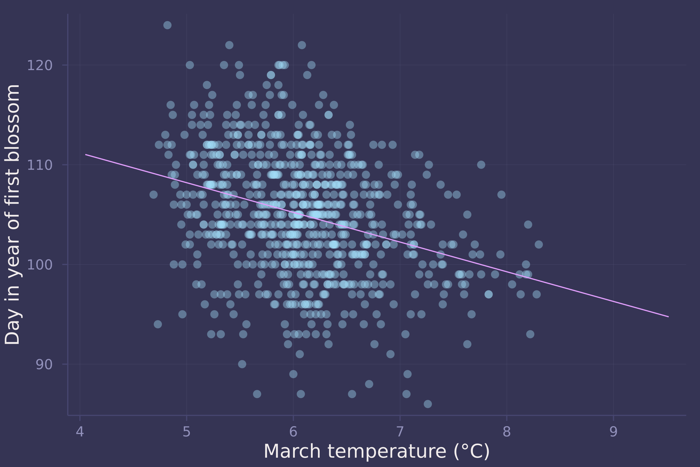
psis_loo(model_line, post_line, source=:mcmc);        # -1074.60
psis_loo(model_splines, post_splines, source=:mcmc);  # -1080.86


temp_seq = collect(range(-3, 5, length=100));
μ_post = post_line["α"] .+ post_line["β"] * temp_seq';

plot(std_temp .* blossoms.temp .+ mean_temp, std_doy .* blossoms.doy .+ mean_doy, ylab="Day in year of first blossom", xlab="March temperature (°C)", seriestype=:scatter, legend=false, alpha=0.4);
plot!(std_temp .* temp_seq .+ mean_temp, std_doy .* vec(mean(μ_post, dims=1)) .+ mean_doy, legend=false)
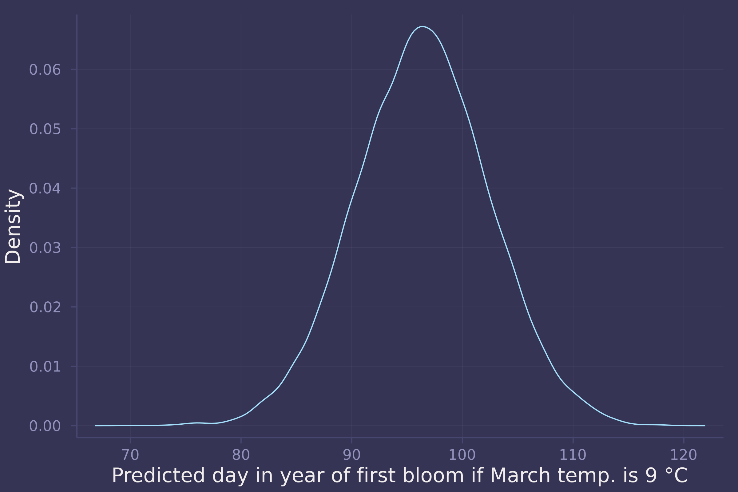
μ_post_at_temp_9C = rand.(Normal.(post_line["α"] .+ post_line["β"] .* (9 .- mean_temp) ./ std_temp, post_line["σ"]));

density(std_doy .* μ_post_at_temp_9C .+ mean_doy, ylab="Density", xlab="Predicted day in year of first bloom if March temp. is 9 °C", legend=false)
Homework 5
1. The data in grants are outcomes for scientific funding applications for the Netherlands Organization for Scientific Research (NWO) from 2010–2012. (see van der Lee and Ellemers <doi:10.1073/pnas.1510159112>). These data have a similar structure to the UCB admissions data discussed in Chapter 11. Draw a DAG for this sample and then use one or more binomial GLMs to estimate the total causal effect of gender on grant awards.
Let G represent the gender of the grant applicant, D represent the discipline of the grant application, and A represent whether or not the grant was awarded.

invlogit(x) = exp(x) / (1 + exp(x));

grants = CSV.read(
    download("https://raw.githubusercontent.com/rmcelreath/rethinking/master/data/NWOGrants.csv"),
    DataFrame,
    delim=';'
)
## 18×4 DataFrame
##  Row │ discipline           gender   applications  awards
##      │ String31             String1  Int64         Int64
## ─────┼────────────────────────────────────────────────────
##    1 │ Chemical sciences    m                  83      22
##    2 │ Chemical sciences    f                  39      10
##    3 │ Physical sciences    m                 135      26
##    4 │ Physical sciences    f                  39       9
##    5 │ Physics              m                  67      18
##    6 │ Physics              f                   9       2
##    7 │ Humanities           m                 230      33
##    8 │ Humanities           f                 166      32
##   ⋮  │          ⋮              ⋮          ⋮          ⋮
##   12 │ Interdisciplinary    f                  78      17
##   13 │ Earth/life sciences  m                 156      38
##   14 │ Earth/life sciences  f                 126      18
##   15 │ Social sciences      m                 425      65
##   16 │ Social sciences      f                 409      47
##   17 │ Medical sciences     m                 245      46
##   18 │ Medical sciences     f                 260      29
##                                             3 rows omitted
grants.gender = [gender == "f" ? 1 : 2 for gender in grants.gender];
disciplines = unique(grants.discipline);
grants.discipline = [
    findfirst(d -> d == discipline, disciplines)
    for discipline in grants.discipline
];

@model function grant_gender_on_award_total(a, g, n)
    α ~ filldist(Normal(0, 1.5), 2)
    p = invlogit.(α[g])
    a .~ Binomial.(n, p)
end;

model_total = grant_gender_on_award_total(
    grants.awards,
    grants.gender,
    grants.applications
);
post_total = sample(model_total, NUTS(), 10_000)
## Chains MCMC chain (10000×14×1 Array{Float64, 3}):
##
## Iterations        = 1001:1:11000
## Number of chains  = 1
## Samples per chain = 10000
## Wall duration     = 7.75 seconds
## Compute duration  = 7.75 seconds
## parameters        = α[1], α[2]
## internals         = lp, n_steps, is_accept, acceptance_rate, log_density, hamiltonian_energy, hamiltonian_energy_error, max_hamiltonian_energy_error, tree_depth, numerical_error, step_size, nom_step_size
##
## Summary Statistics
##   parameters      mean       std   naive_se      mcse          ess      rhat   ⋯
##       Symbol   Float64   Float64    Float64   Float64      Float64   Float64   ⋯
##
##         α[1]   -1.7383    0.0823     0.0008    0.0009    9852.4335    0.9999   ⋯
##         α[2]   -1.5330    0.0644     0.0006    0.0005   10554.9990    1.0000   ⋯
##                                                                 1 column omitted
##
## Quantiles
##   parameters      2.5%     25.0%     50.0%     75.0%     97.5%
##       Symbol   Float64   Float64   Float64   Float64   Float64
##
##         α[1]   -1.9014   -1.7942   -1.7368   -1.6832   -1.5792
##         α[2]   -1.6601   -1.5769   -1.5320   -1.4894   -1.4077
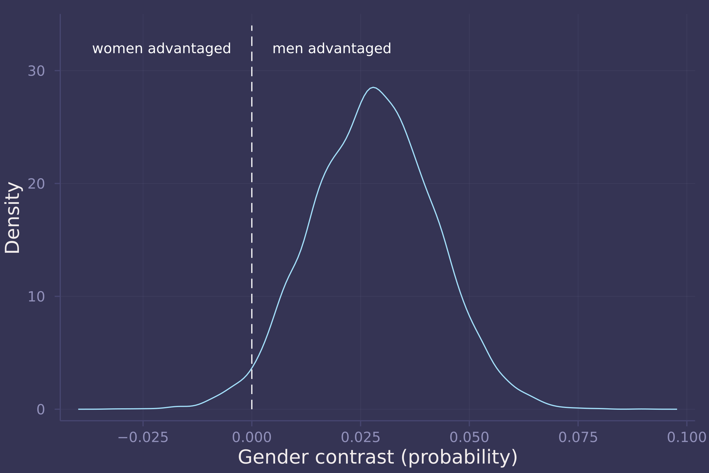
gender_adv_total = invlogit.(post_total["α[2]"]) - invlogit.(post_total["α[1]"]);

density(gender_adv_total, ylab="Density", xlab="Gender contrast (probability)", legend=false);
plot!([0, 0], [0, 34], line=:dash, color=:white);
annotate!(-0.005, 32, text("women advantaged", :white, :right, 8));
annotate!(0.005, 32, text("men advantaged", :white, :left, 8))
2. Now estimate the direct causal effect of gender on grant awards. Compute the average direct causal effect of gender, weighting each discipline in proportion to the number of applications in the sample. Refer to the marginal effect example in Lecture 9 for help.
@model function grant_gender_on_award_direct(a, g, n, d)
    α ~ filldist(Normal(0, 1.5), length(unique(g)), length(unique(d)))
    for i in 1:length(a)
        a[i] ~ Binomial(n[i], invlogit(α[g[i], d[i]]))
    end
end;

model_direct = grant_gender_on_award_direct(
    grants.awards,
    grants.gender,
    grants.applications,
    grants.discipline
);
post_direct = sample(model_direct, NUTS(), 10_000)
## Chains MCMC chain (10000×30×1 Array{Float64, 3}):
##
## Iterations        = 1001:1:11000
## Number of chains  = 1
## Samples per chain = 10000
## Wall duration     = 4.78 seconds
## Compute duration  = 4.78 seconds
## parameters        = α[1,1], α[2,1], α[1,2], α[2,2], α[1,3], α[2,3], α[1,4], α[2,4], α[1,5], α[2,5], α[1,6], α[2,6], α[1,7], α[2,7], α[1,8], α[2,8], α[1,9], α[2,9]
## internals         = lp, n_steps, is_accept, acceptance_rate, log_density, hamiltonian_energy, hamiltonian_energy_error, max_hamiltonian_energy_error, tree_depth, numerical_error, step_size, nom_step_size
##
## Summary Statistics
##   parameters      mean       std   naive_se      mcse          ess      rhat   ⋯
##       Symbol   Float64   Float64    Float64   Float64      Float64   Float64   ⋯
##
##       α[1,1]   -1.0354    0.3565     0.0036    0.0027   17314.5238    0.9999   ⋯
##       α[2,1]   -1.0055    0.2426     0.0024    0.0017   16975.3056    1.0001   ⋯
##       α[1,2]   -1.1640    0.3646     0.0036    0.0030   14896.8231    1.0000   ⋯
##       α[2,2]   -1.4197    0.2212     0.0022    0.0018   15476.4679    0.9999   ⋯
##       α[1,3]   -1.0686    0.6990     0.0070    0.0053   16916.5101    0.9999   ⋯
##       α[2,3]   -0.9901    0.2763     0.0028    0.0023   16650.9139    0.9999   ⋯
##       α[1,4]   -1.4195    0.1938     0.0019    0.0016   18235.8213    0.9999   ⋯
##       α[2,4]   -1.7713    0.1867     0.0019    0.0014   15472.5930    0.9999   ⋯
##       α[1,5]   -1.2981    0.3077     0.0031    0.0022   16814.2082    0.9999   ⋯
##       α[2,5]   -1.6534    0.1953     0.0020    0.0015   16313.0272    0.9999   ⋯
##       α[1,6]   -1.2575    0.2727     0.0027    0.0021   17493.6539    1.0001   ⋯
##       α[2,6]   -1.9976    0.2970     0.0030    0.0024   17122.6507    1.0001   ⋯
##       α[1,7]   -1.7645    0.2512     0.0025    0.0016   19403.7417    0.9999   ⋯
##       α[2,7]   -1.1263    0.1853     0.0019    0.0014   20398.8360    0.9999   ⋯
##       α[1,8]   -2.0284    0.1535     0.0015    0.0014   14443.1747    0.9999   ⋯
##       α[2,8]   -1.7047    0.1320     0.0013    0.0009   17872.9843    0.9999   ⋯
##       α[1,9]   -2.0521    0.1935     0.0019    0.0014   20877.7466    0.9999   ⋯
##       α[2,9]   -1.4575    0.1642     0.0016    0.0012   19516.6949    0.9999   ⋯
##                                                                 1 column omitted
##
## Quantiles
##   parameters      2.5%     25.0%     50.0%     75.0%     97.5%
##       Symbol   Float64   Float64   Float64   Float64   Float64
##
##       α[1,1]   -1.7650   -1.2663   -1.0244   -0.7895   -0.3700
##       α[2,1]   -1.4856   -1.1677   -1.0000   -0.8394   -0.5447
##       α[1,2]   -1.9138   -1.3993   -1.1510   -0.9162   -0.4844
##       α[2,2]   -1.8670   -1.5689   -1.4159   -1.2702   -0.9980
##       α[1,3]   -2.5336   -1.5215   -1.0411   -0.5953    0.2414
##       α[2,3]   -1.5518   -1.1774   -0.9813   -0.8001   -0.4703
##       α[1,4]   -1.8128   -1.5487   -1.4144   -1.2878   -1.0526
##       α[2,4]   -2.1513   -1.8963   -1.7662   -1.6446   -1.4145
##       α[1,5]   -1.9183   -1.4995   -1.2913   -1.0873   -0.7207
##       α[2,5]   -2.0521   -1.7784   -1.6465   -1.5223   -1.2849
##       α[1,6]   -1.8120   -1.4371   -1.2509   -1.0728   -0.7437
##       α[2,6]   -2.6055   -2.1927   -1.9856   -1.7926   -1.4437
##       α[1,7]   -2.2604   -1.9313   -1.7592   -1.5887   -1.2964
##       α[2,7]   -1.4985   -1.2483   -1.1249   -1.0006   -0.7719
##       α[1,8]   -2.3439   -2.1274   -2.0226   -1.9249   -1.7398
##       α[2,8]   -1.9689   -1.7928   -1.7031   -1.6146   -1.4503
##       α[1,9]   -2.4342   -2.1809   -2.0468   -1.9189   -1.6866
##       α[2,9]   -1.7929   -1.5640   -1.4528   -1.3469   -1.1426
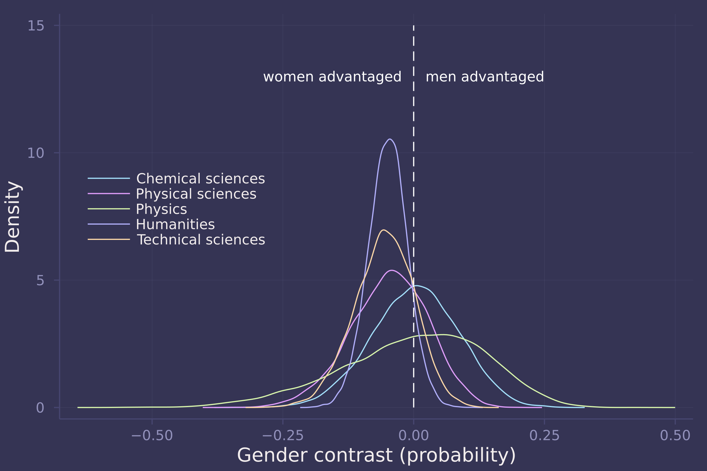
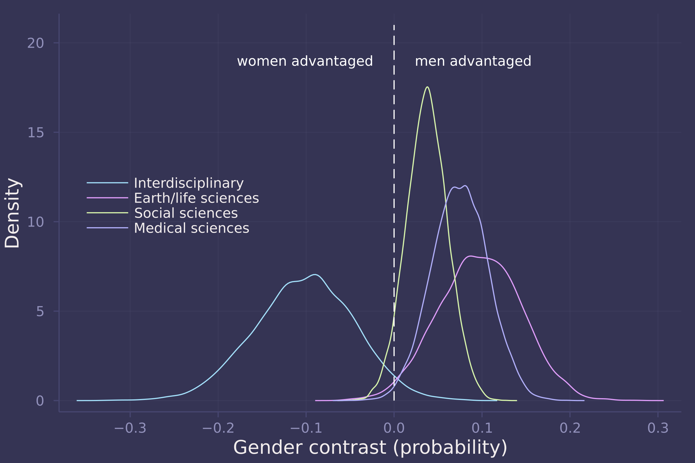
gender_adv_direct = [
    invlogit.(post_direct["α[2,$i]"]) -
    invlogit.(post_direct["α[1,$i]"])
    for i in 1:length(disciplines)
];
gender_adv_direct = hcat(gender_adv_direct...);

density(gender_adv_direct[:, 1:5], ylab="Density", xlab="Gender contrast (probability)", labels=["Chemical sciences" "Physical sciences" "Physics" "Humanities" "Technical sciences"], legend=:left);
plot!([0, 0], [0, 15], line=:dash, color=:white, label="");
annotate!(-0.025, 13, text("women advantaged", :white, :right, 8));
annotate!(0.025, 13, text("men advantaged", :white, :left, 8))
density(gender_adv_direct[:, 6:9], ylab="Density", xlab="Gender contrast (probability)", labels=["Interdisciplinary" "Earth/life sciences" "Social sciences" "Medical sciences"], legend=:left);
plot!([0, 0], [0, 21], line=:dash, color=:white, label="");
annotate!(-0.025, 19, text("women advantaged", :white, :right, 8));
annotate!(0.025, 19, text("men advantaged", :white, :left, 8))
3. Considering the total effect (problem 1) and direct effect (problem 2) of gender, what causes contribute to the average difference between women and men in award rate in this sample? It is not necessary to say whether or not there is evidence of discrimination. Simply explain how the direct effects you have estimated make sense (or not) of the total effect.
Homework 6
The theme of this homework is tadpoles. You must keep them alive.
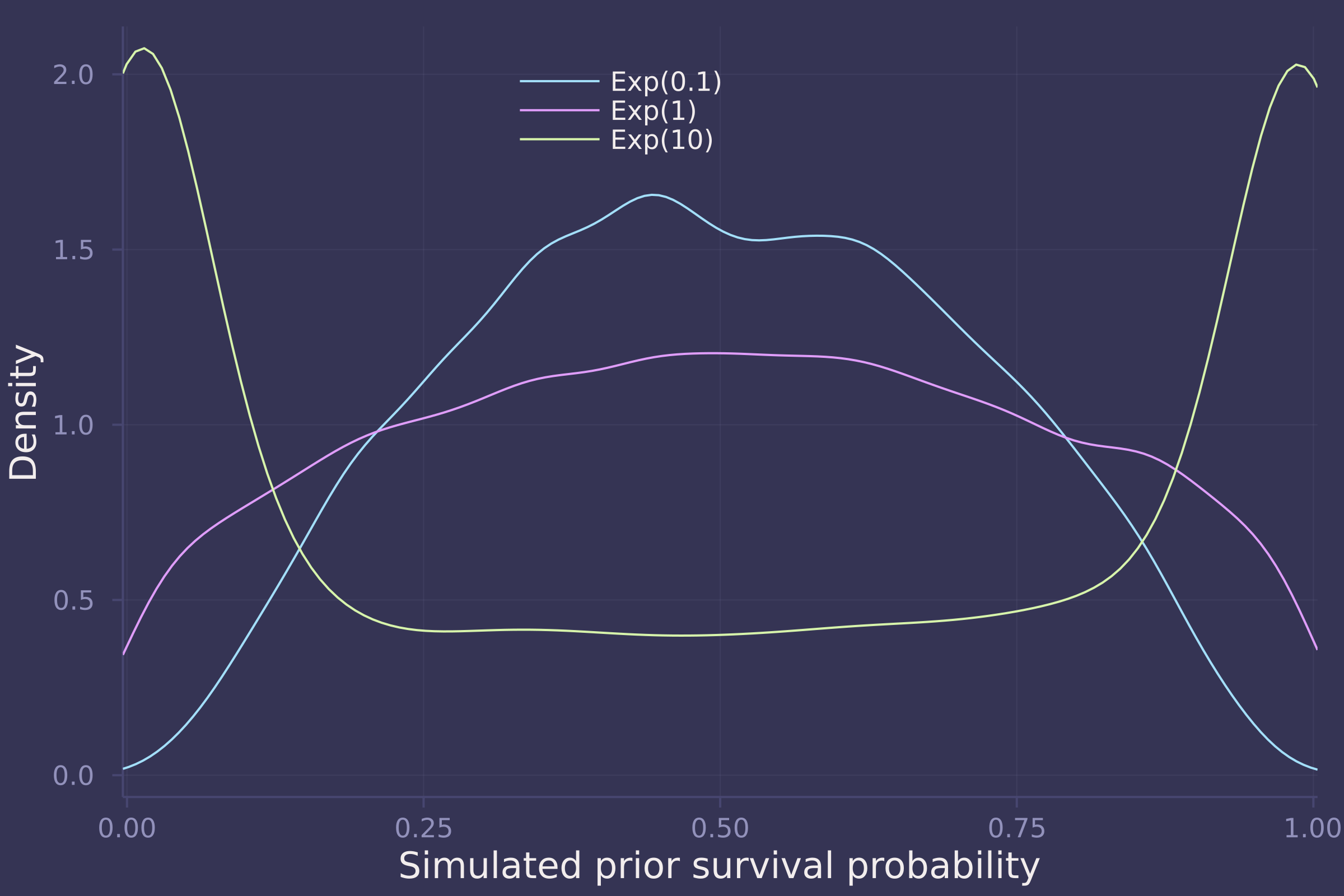
1. Conduct a prior predictive simulation for the Reedfrog model. By this I mean to simulate the prior distribution of tank survival probabilities αj . Start by using this prior:
Be sure to transform the αj values to the probability scale for plotting and summary. How does increasing the width of the prior on σ change the prior distribution αj ? You might try Exponential(10) and Exponential(0.1) for example.
# redefine a version of invlogit that's more computationally stable
invlogit(x) = exp(x - log(1 + exp(x)));

σ_dists = [Exponential(0.1), Exponential(1), Exponential(10)];

function sim_priors(σ_dist, n=10_000)
    σ = rand(σ_dist, n)
    ᾱ = rand(Normal(0, 1), n)
    α = rand.(Normal.(ᾱ, σ))
    invlogit.(α)
end;

sims = hcat(sim_priors.(σ_dists)...);

density(sims, xlims=[0.025, 0.975], ylab="Density",xlab="Simulated prior survival probability", labels=["Exp(0.1)" "Exp(1)" "Exp(10)"], legend=:top)
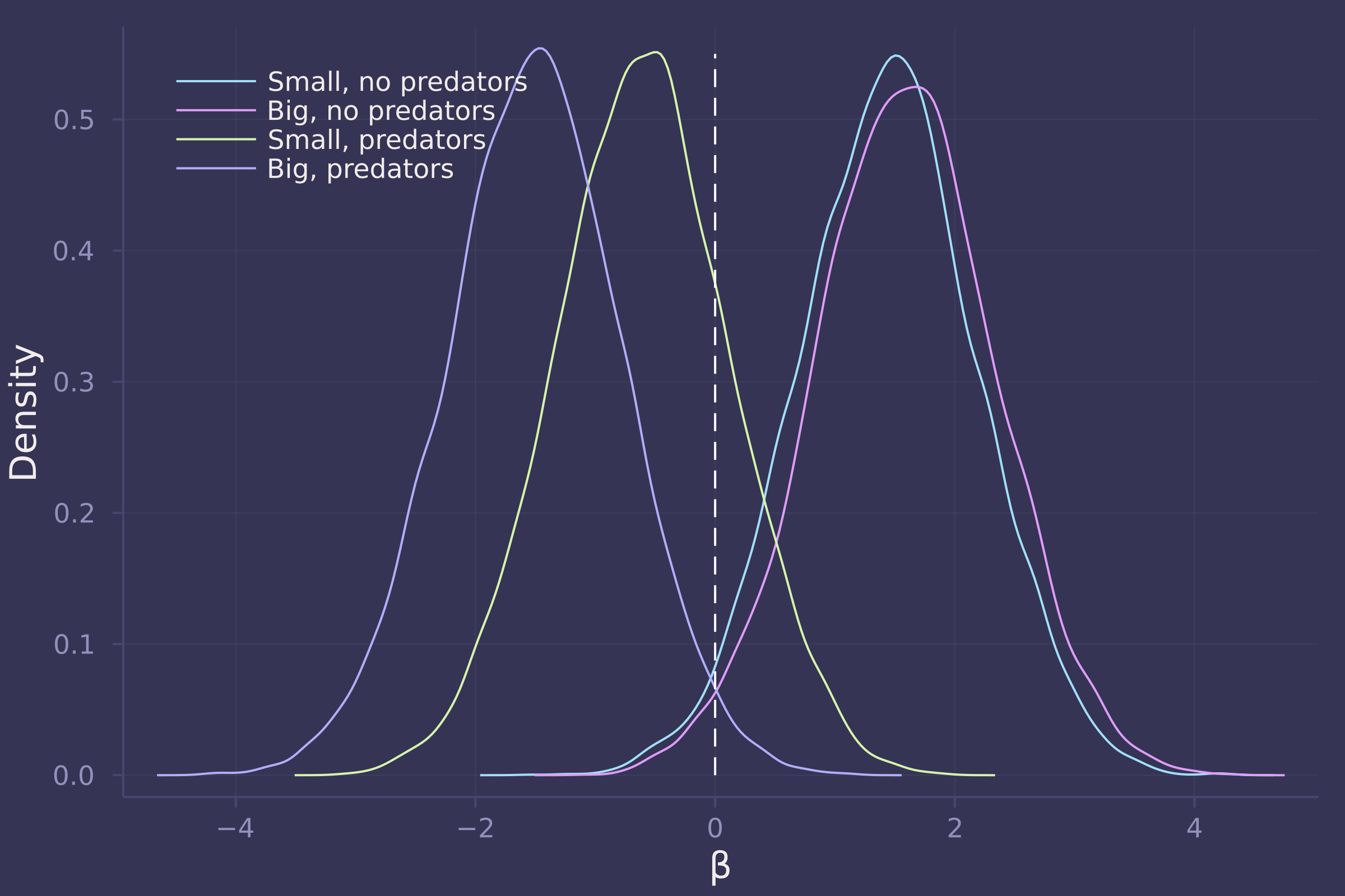
2. Revisit the Reedfrog survival data. Start with the varying effects model from the book and the lecture. Then modify it to estimate the causal effects of the treatement variables pred and size, including how size might modify the effect of predation. An easy approach is to estimate the effect for each combination of pred and size. Justify your model with a DAG of this experiment.
tadpoles = CSV.read(
    download("https://raw.githubusercontent.com/rmcelreath/rethinking/master/data/reedfrogs.csv"),
    DataFrame,
    delim=';'
)
## 48×5 DataFrame
##  Row │ density  pred     size     surv   propsurv
##      │ Int64    String7  String7  Int64  Float64
## ─────┼────────────────────────────────────────────
##    1 │      10  no       big          9  0.9
##    2 │      10  no       big         10  1.0
##    3 │      10  no       big          7  0.7
##    4 │      10  no       big         10  1.0
##    5 │      10  no       small        9  0.9
##    6 │      10  no       small        9  0.9
##    7 │      10  no       small       10  1.0
##    8 │      10  no       small        9  0.9
##   ⋮  │    ⋮        ⋮        ⋮       ⋮       ⋮
##   42 │      35  pred     big         12  0.342857
##   43 │      35  pred     big         13  0.371429
##   44 │      35  pred     big         14  0.4
##   45 │      35  pred     small       22  0.628571
##   46 │      35  pred     small       12  0.342857
##   47 │      35  pred     small       31  0.885714
##   48 │      35  pred     small       17  0.485714
##                                    33 rows omitted
tadpoles.tank = collect(1:size(tadpoles, 1));
tadpoles.pred = [pred == "no" ? 1 : 2 for pred in tadpoles.pred];
tadpoles.size = [size == "small" ? 1 : 2 for size in tadpoles.size];
@model function survival_vareff(surv, density, tank, pred, size)
    σ ~ Exponential(1)
    ᾱ ~ Normal(0, 1.5)
    α ~ filldist(Normal(ᾱ, σ), length(unique(tank)))
    β ~ filldist(Normal(0, 1.5), length(unique(pred)), length(unique(size)))
    for i in 1:length(surv)
        surv[i] ~ Binomial(density[i], invlogit(α[i] + β[pred[i], size[i]]))
    end
end;

model_vareff = survival_vareff(
    tadpoles.surv,
    tadpoles.density,
    tadpoles.tank,
    tadpoles.pred,
    tadpoles.size
);
post_vareff = sample(model_vareff, NUTS(), 10_000);
βs = ["β[1,1]", "β[1,2]", "β[2,1]", "β[2,2]"];

density([post_vareff[β] for β in βs], ylab="Density", xlab="β", labels=["Small, no predators" "Big, no predators" "Small, predators" "Big, predators"], legend=:topleft);
plot!([0, 0], [0, 0.55], line=:dash, color=:white, label="")
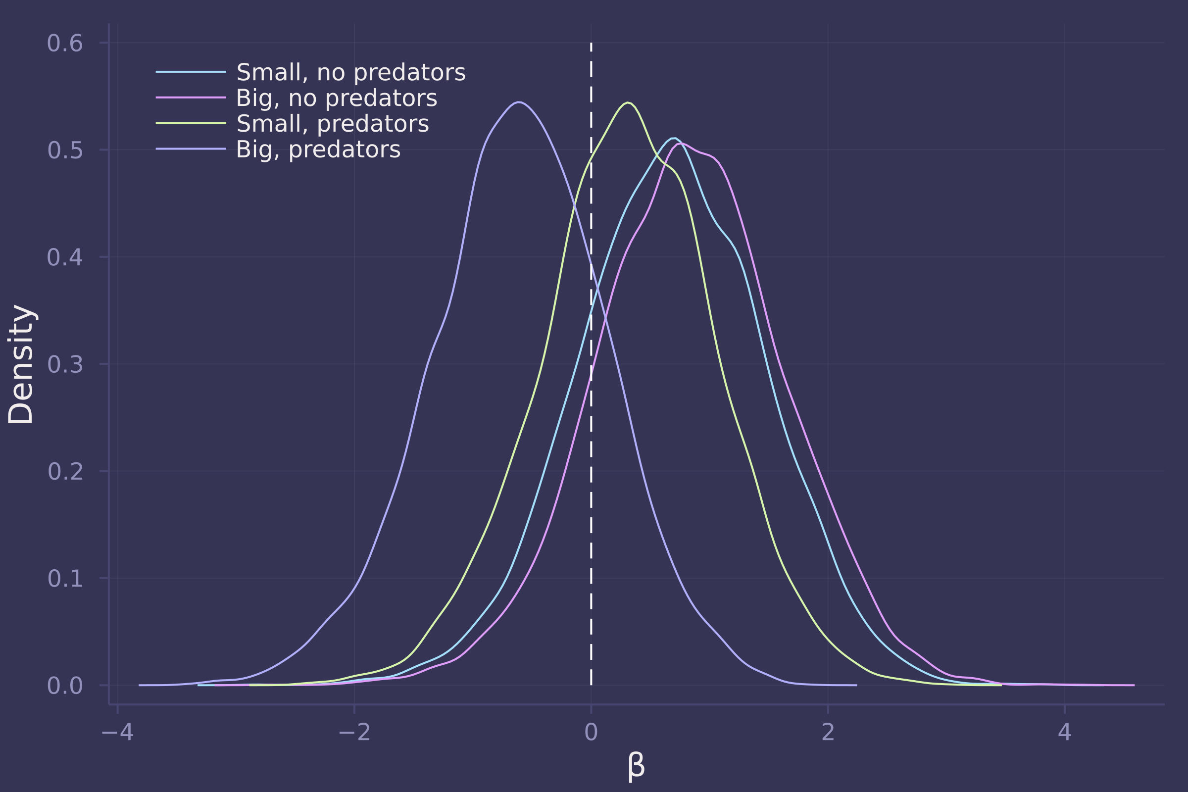
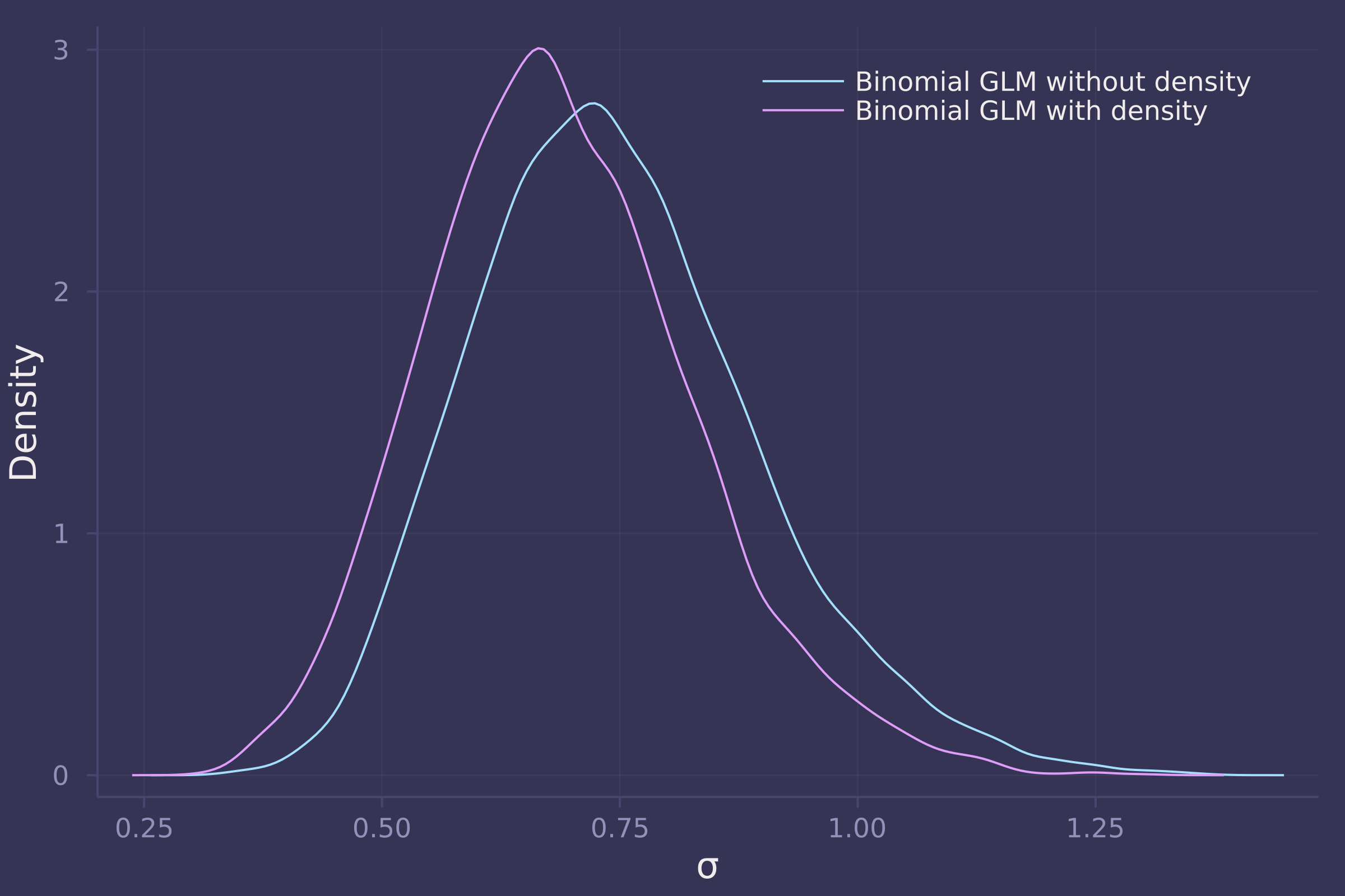
3. Now estimate the causal effect of density on survival. Consider whether pred modifies the effect of density. There are several good ways to include density in your Binomial GLM. You could treat it as a continuous regression variable (possibly standardized). Or you could convert it to an ordered category (with three levels). Compare the σ (tank standard deviation) posterior distribution to σ from your model in Problem 2. How are they different? Why?
@model function survival_with_density(surv, density, tank, pred, size)
    σ ~ Exponential(1)
    ᾱ ~ Normal(0, 1.5)
    α ~ filldist(Normal(ᾱ, σ), length(unique(tank)))
    β ~ filldist(Normal(0, 1.5), length(unique(pred)), length(unique(size)))
    γ ~ filldist(Normal(0, 1.5), length(unique(pred)))
    for i in 1:length(surv)
        surv[i] ~ Binomial(density[i], invlogit(α[i] + β[pred[i], size[i]] + γ[pred[i]] * density[i]))
    end
end;

model_with_density = survival_with_density(
    tadpoles.surv,
    tadpoles.density,
    tadpoles.tank,
    tadpoles.pred,
    tadpoles.size
);
post_with_density = sample(model_with_density, NUTS(), 10_000);
βs = ["β[1,1]", "β[1,2]", "β[2,1]", "β[2,2]"];

density([post_with_density[β] for β in βs], ylab="Density", xlab="β", labels=["Small, no predators" "Big, no predators" "Small, predators" "Big, predators"], legend=:topleft);
plot!([0, 0], [0, 0.6], line=:dash, color=:white, label="")
γs = ["γ[1]", "γ[2]"];

density([post_with_density[γ] for γ in γs], ylab="Density", xlab="γ", labels=["No predators" "Predators"], legend=:topleft);
plot!([0, 0], [0, 30], line=:dash, color=:white, label="")
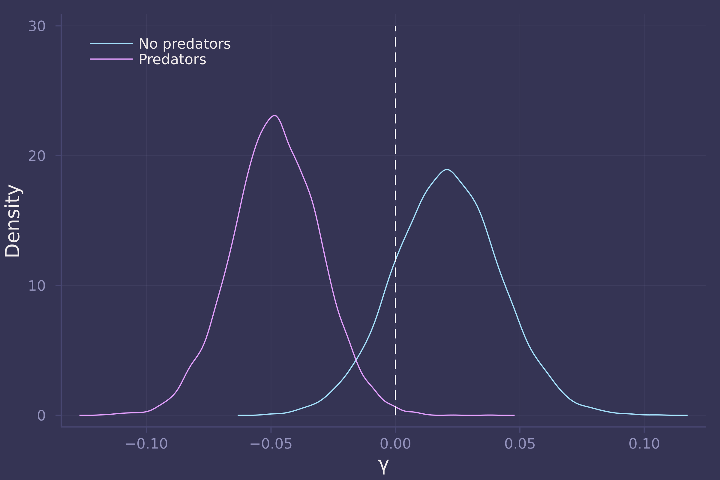
density([post_vareff["σ"], post_with_density["σ"]], ylab="Density", xlab="σ", labels=["Binomial GLM without density" "Binomial GLM with density"])
Homework 7
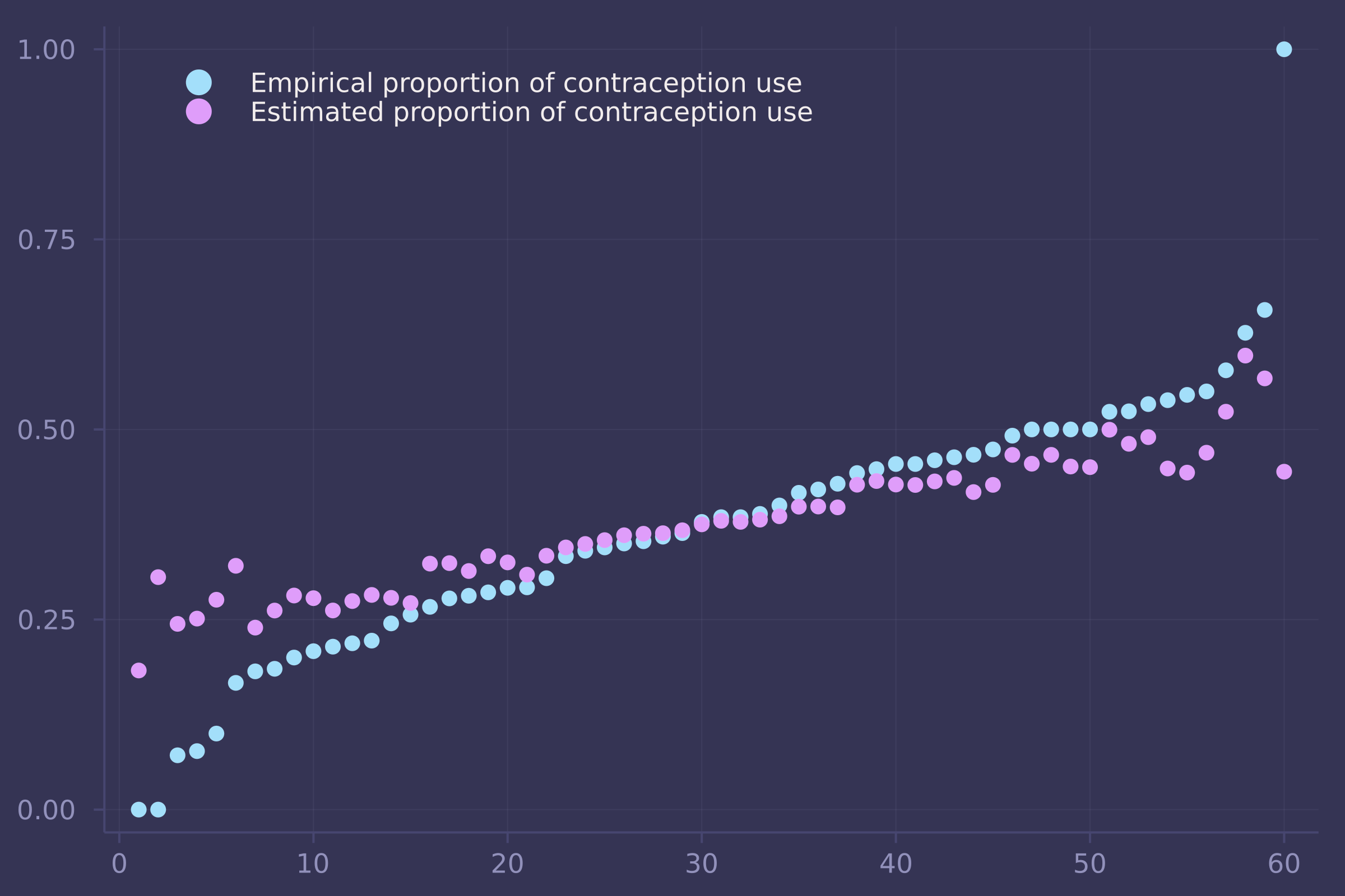
1. The data in bangladesh are 1934 women from the 1989 Bangladesh Fertility Survey. For each woman, we know which district she lived, her number of living_children, her age_centered, whether she lived in an urban center, and finally whether or not she used contraception (use_contraception). In the first problem, I only want you to investigate the proportion of women using contraception in each distirct. Use partial pooling (varying effects). Then compare the varying effects estimates to the raw empirical proportion in each district. Explain the differences between the estimates and the data. Note that district number 54 is absent in the data. This may cause some problems in indexing the parameters. Pay special attention to district number 54’s estimate.
bangladesh = CSV.read(
    download("https://raw.githubusercontent.com/rmcelreath/rethinking/master/data/bangladesh.csv"),
    DataFrame,
    delim=';'
);

rename!(
    bangladesh,
    "use.contraception" => :use_contraception,
    "living.children" => :living_children,
    "age.centered" => :age_centered
)
## 1934×6 DataFrame
##   Row │ woman  district  use_contraception  living_children  age_centered  urb ⋯
##       │ Int64  Int64     Int64              Int64            Float64       Int ⋯
## ──────┼─────────────────────────────────────────────────────────────────────────
##     1 │     1         1                  0                4       18.44        ⋯
##     2 │     2         1                  0                1       -5.5599
##     3 │     3         1                  0                3        1.44
##     4 │     4         1                  0                4        8.44
##     5 │     5         1                  0                1      -13.559       ⋯
##     6 │     6         1                  0                1      -11.56
##     7 │     7         1                  0                4       18.44
##     8 │     8         1                  0                4       -3.5599
##   ⋮   │   ⋮       ⋮              ⋮                 ⋮              ⋮          ⋮ ⋱
##  1928 │  1928        61                  1                3       -9.5599      ⋯
##  1929 │  1929        61                  0                3       -2.5599
##  1930 │  1930        61                  0                4       14.44
##  1931 │  1931        61                  0                3       -4.5599
##  1932 │  1932        61                  0                4       14.44        ⋯
##  1933 │  1933        61                  0                1      -13.56
##  1934 │  1934        61                  0                4       10.44
##                                                   1 column and 1919 rows omitted
bangladesh_districts = combine(
    groupby(bangladesh, :district),
    :woman => length => :n_total,
    :use_contraception => sum => :n_use_contraception
)
## 60×3 DataFrame
##  Row │ district  n_total  n_use_contraception
##      │ Int64     Int64    Int64
## ─────┼────────────────────────────────────────
##    1 │        1      117                   30
##    2 │        2       20                    7
##    3 │        3        2                    2
##    4 │        4       30                   15
##    5 │        5       39                   14
##    6 │        6       65                   19
##    7 │        7       18                    5
##    8 │        8       37                   14
##   ⋮  │    ⋮         ⋮              ⋮
##   54 │       55        6                    1
##   55 │       56       45                   26
##   56 │       57       27                    5
##   57 │       58       33                   15
##   58 │       59       10                    1
##   59 │       60       32                    7
##   60 │       61       42                    9
##                                45 rows omitted
@model function bangladesh_district_contraception_use(d, n, k)
    σ ~ Exponential(1)
    ᾱ ~ Normal(0, 1.5)
    α ~ filldist(Normal(ᾱ, σ), length(d))
    k .~ Binomial.(n, invlogit.(α))
end;

model_bangladesh_district_contraception_use = bangladesh_district_contraception_use(
    bangladesh_districts.district,
    bangladesh_districts.n_total,
    bangladesh_districts.n_use_contraception
);
post_bangladesh_district_contraception_use = sample(
    model_bangladesh_district_contraception_use,
    NUTS(),
    10_000
);
post_p = invlogit.(
    post_bangladesh_district_contraception_use[["α[$i]" for i in 1:length(bangladesh_districts.district)]].value
);

p_df = DataFrame(
    district = bangladesh_districts.district,
    estimate = vec(mean(post_p, dims=1)),
    empirical = bangladesh_districts.n_use_contraception ./ bangladesh_districts.n_total
);
sort!(p_df, :empirical)
## 60×3 DataFrame
##  Row │ district  estimate  empirical
##      │ Int64     Float64   Float64
## ─────┼───────────────────────────────
##    1 │       11  0.182979  0.0
##    2 │       49  0.30574   0.0
##    3 │       24  0.244268  0.0714286
##    4 │       10  0.251211  0.0769231
##    5 │       59  0.276014  0.1
##    6 │       55  0.320645  0.166667
##    7 │       27  0.23933   0.181818
##    8 │       57  0.261808  0.185185
##   ⋮  │    ⋮         ⋮          ⋮
##   54 │       37  0.448628  0.538462
##   55 │       42  0.443219  0.545455
##   56 │       16  0.46939   0.55
##   57 │       56  0.52331   0.577778
##   58 │       14  0.597111  0.627119
##   59 │       34  0.567127  0.657143
##   60 │        3  0.444418  1.0
##                       45 rows omitted
plot(1:nrow(p_df), [p_df.empirical p_df.estimate], seriestype=:scatter, labels=["Empirical proportion of contraception use" "Estimated proportion of contraception use"], legend=:topleft)
2. First, draw a DAG that includes all five variables. Use contraception C , Age A , Children K , Urban U , and District D . You don’t have to be an expert on fertility. But do think about which variables can influence which other variables. Second, design an estimation strategy to identify both the total and direct causal effects of living in an urban center on contraceptive use. Those are your estimands. Consider causal relationships among the variables. Then use your DAG to justify an adjustment set that will yield the estimate of the causal effect of urban living on contraceptive use. Do not run a statistical model (yet). I just want you to try to design an analysis. There is no firm right answer. Just apply the backdoor criterion and rules of d-separation (the elemental confounds) correctly to the DAG you design.

3. Now build one or more statistical models to estimate the total and the direct causal effects of urban living on contraceptive use. Again include district as a simple varying effect (as in problem 1) so that each district has its own average contraceptive use. You may also want to stratify the effect of urban living by district. If you do, think carefully about how to do this statistically.
@model function bangladesh_urban_on_contraception_use_total(c, u, d, n_districts)
σ ~ Exponential(1)
ᾱ ~ Normal(0, 1.5)
α ~ filldist(Normal(ᾱ, σ), n_districts)
β ~ Normal(0, 0.5)
for i in 1:length(c)
c[i] ~ Bernoulli(invlogit(α[d[i]] + β * u[i]))
end
end;
model_bangladesh_urban_on_contraception_use_total = bangladesh_urban_on_contraception_use_total(
bangladesh.use_contraception,
bangladesh.urban,
bangladesh.district,
maximum(bangladesh.district)
);
post_bangladesh_urban_on_contraception_use_total = sample(
model_bangladesh_urban_on_contraception_use_total,
NUTS(),
5_000
);
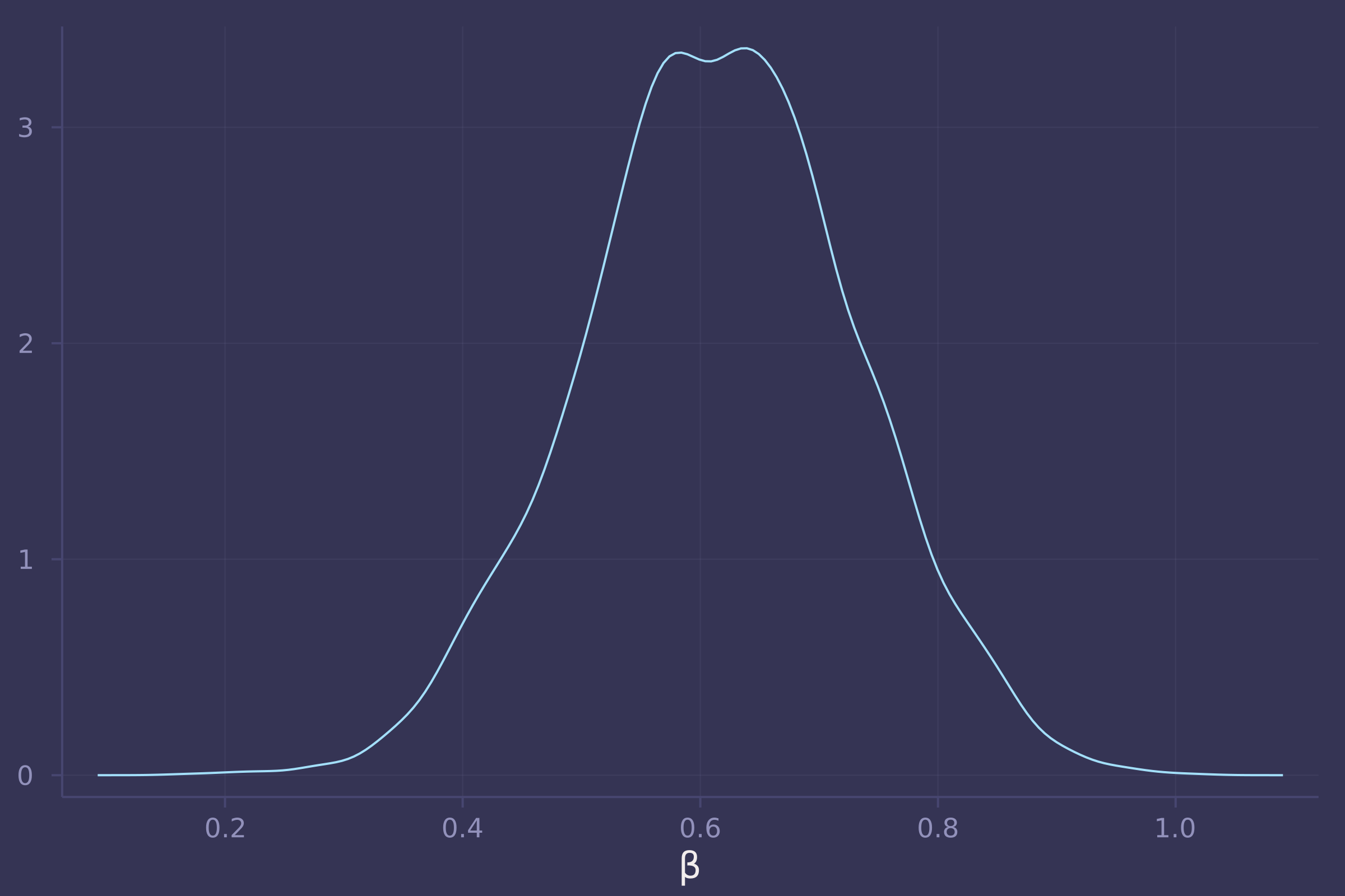
density(post_bangladesh_urban_on_contraception_use_total[:β], xlab="β", legend=false)
@model function bangladesh_urban_on_contraception_use_direct(c, u, d, a, k, n_districts)
σ ~ Exponential(1)
ᾱ ~ Normal(0, 1.5)
α ~ filldist(Normal(ᾱ, σ), n_districts)
β ~ Normal(0, 0.5)
γ ~ Normal(0, 0.5)
δ ~ Dirichlet(length(unique(k)), 2)
for i in 1:length(c)
c[i] ~ Bernoulli(invlogit(α[d[i]] + β * u[i] + γ * a[i] + δ[k[i]]))
end
end;
model_bangladesh_urban_on_contraception_use_direct = bangladesh_urban_on_contraception_use_direct(
bangladesh.use_contraception,
bangladesh.urban,
bangladesh.district,
standardize(bangladesh.age_centered),
bangladesh.living_children,
maximum(bangladesh.district)
);
post_bangladesh_urban_on_contraception_use_direct = sample(
model_bangladesh_urban_on_contraception_use_direct,
NUTS(),
5_000
);
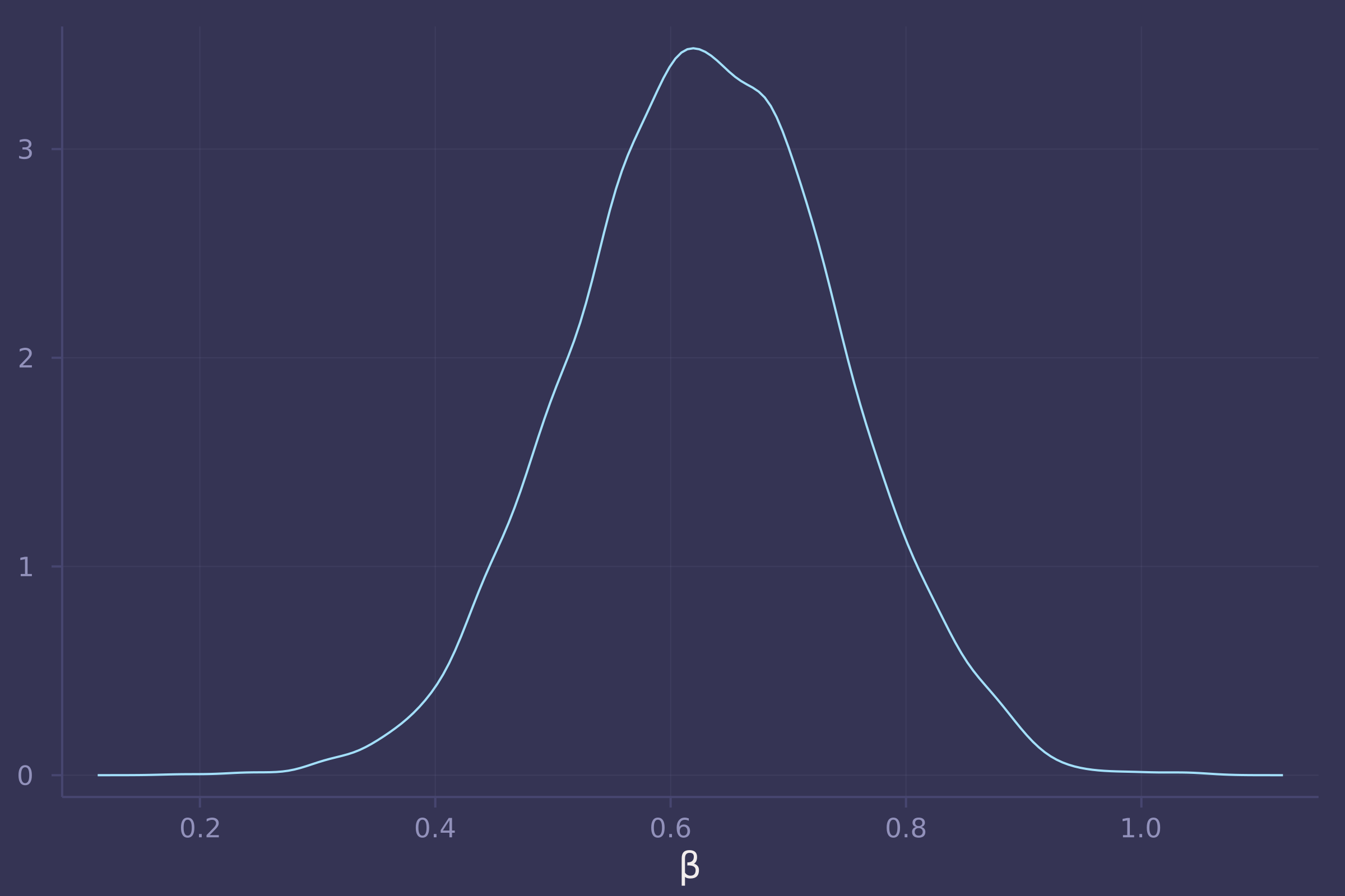
density(post_bangladesh_urban_on_contraception_use_direct[:β], xlab="β", legend=false)
Homework 8
This assignment is difficult to complete without support for LKJCholesky in Turing.jl. There is an open issue to address this at github.com/TuringLang/Turing.jl/issues/1629.
invlogit(x) = 1 ./ (exp(-x) .+ 1);

monks = CSV.read(
    download("https://raw.githubusercontent.com/rmcelreath/stat_rethinking_2022/main/homework/week08_Monks.csv"),
    DataFrame
)
## 153×9 DataFrame
##  Row │ dyad_id  A      B      like_AB  like_BA  dislike_AB  dislike_BA  A_name ⋯
##      │ Int64    Int64  Int64  Int64    Int64    Int64       Int64       String ⋯
## ─────┼──────────────────────────────────────────────────────────────────────────
##    1 │       1      1      2        0        3           0           0  ROMUL  ⋯
##    2 │       2      1      3        3        3           0           0  ROMUL
##    3 │       3      1      4        0        0           0           0  ROMUL
##    4 │       4      1      5        0        0           0           0  ROMUL
##    5 │       5      1      6        0        0           0           0  ROMUL  ⋯
##    6 │       6      1      7        0        0           0           0  ROMUL
##    7 │       7      1      8        0        0           0           0  ROMUL
##    8 │       8      1      9        0        0           0           1  ROMUL
##   ⋮  │    ⋮       ⋮      ⋮       ⋮        ⋮         ⋮           ⋮          ⋮   ⋱
##  147 │     147     14     18        0        0           0           0  ALBERT ⋯
##  148 │     148     15     16        0        1           0           0  AMAND
##  149 │     149     15     17        0        0           0           0  AMAND
##  150 │     150     15     18        0        0           0           0  AMAND
##  151 │     151     16     17        0        0           0           0  BASIL  ⋯
##  152 │     152     16     18        0        0           0           0  BASIL
##  153 │     153     17     18        3        3           0           0  ELIAS
##                                                   2 columns and 138 rows omitted
@model function monk_reciprocity(like_ab, like_ba, dyad_id, n_dyads)
    σ ~ Exponential(1)
    P ~ LKJ(2, 1)
    d = Matrix(undef, n_dyads, 2)
    for i in 1:n_dyads
        d[i, :] = σ .* cholesky(P).L * randn(2)
    end
    α ~ Normal(0, 1)
    p_ab = invlogit.(α .+ d[:, 1])
    p_ba = invlogit.(α .+ d[:, 2])
    like_ab .~ Binomial.(3, p_ab)
    like_ba .~ Binomial.(3, p_ba)
end;

model_monk_reciprocity = monk_reciprocity(
    monks.like_AB,
    monks.like_BA,
    monks.dyad_id,
    nrow(monks)
);
@time post_monk_reciprocity = sample(model_monk_reciprocity, NUTS(), 500)
## 200.584295 seconds (2.73 G allocations: 283.401 GiB, 19.40% gc time, 0.01% compilation time)

## Chains MCMC chain (500×18×1 Array{Float64, 3}):
##
## Iterations        = 251:1:750
## Number of chains  = 1
## Samples per chain = 500
## Wall duration     = 187.29 seconds
## Compute duration  = 187.29 seconds
## parameters        = σ, P[1,1], P[2,1], P[1,2], P[2,2], α
## internals         = lp, n_steps, is_accept, acceptance_rate, log_density, hamiltonian_energy, hamiltonian_energy_error, max_hamiltonian_energy_error, tree_depth, numerical_error, step_size, nom_step_size
##
## Summary Statistics
##   parameters      mean       std   naive_se      mcse       ess      rhat   es ⋯
##       Symbol   Float64   Float64    Float64   Float64   Float64   Float64      ⋯
##
##            σ    0.3219    0.0000     0.0000    0.0000    2.0080    0.9980      ⋯
##       P[1,1]    1.0000    0.0000     0.0000    0.0000       NaN       NaN      ⋯
##       P[2,1]   -0.5501    0.0000     0.0000    0.0000       NaN       NaN      ⋯
##       P[1,2]   -0.5501    0.0000     0.0000    0.0000       NaN       NaN      ⋯
##       P[2,2]    1.0000    0.0000     0.0000    0.0000    2.0080    0.9980      ⋯
##            α   -1.8666    0.0000     0.0000    0.0000    2.0080    0.9980      ⋯
##                                                                 1 column omitted
##
## Quantiles
##   parameters      2.5%     25.0%     50.0%     75.0%     97.5%
##       Symbol   Float64   Float64   Float64   Float64   Float64
##
##            σ    0.3219    0.3219    0.3219    0.3219    0.3219
##       P[1,1]    1.0000    1.0000    1.0000    1.0000    1.0000
##       P[2,1]   -0.5501   -0.5501   -0.5501   -0.5501   -0.5501
##       P[1,2]   -0.5501   -0.5501   -0.5501   -0.5501   -0.5501
##       P[2,2]    1.0000    1.0000    1.0000    1.0000    1.0000
##            α   -1.8666   -1.8666   -1.8666   -1.8666   -1.8666
Homework 9
trips = CSV.read(
    download("https://raw.githubusercontent.com/rmcelreath/rethinking/master/data/Achehunting.csv"),
    DataFrame,
    delim=';'
)
## 14364×8 DataFrame
##    Row │ month  day     year   id     age    kg.meat  hours       datatype
##        │ Int64  Int64?  Int64  Int64  Int64  Float64  Float64?    Float64
## ───────┼───────────────────────────────────────────────────────────────────
##      1 │    10       2   1981   3043     67     0.0         6.97       1.0
##      2 │    10       3   1981   3043     67     0.0         9.0        1.0
##      3 │    10       4   1981   3043     67     0.0         1.55       1.0
##      4 │    10       5   1981   3043     67     4.5         8.0        1.0
##      5 │    10       6   1981   3043     67     0.0         3.0        1.0
##      6 │    10       7   1981   3043     67     0.0         7.5        1.0
##      7 │    10       8   1981   3043     67     0.0         9.0        1.0
##      8 │     2       6   1982   3043     68     0.0         7.3        1.0
##    ⋮   │   ⋮      ⋮       ⋮      ⋮      ⋮       ⋮         ⋮          ⋮
##  14358 │     8      26   2006  60121     21     4.96  missing          3.0
##  14359 │     8      27   2006  60121     21     0.0   missing          3.0
##  14360 │     2       2   2007  60121     22     0.0   missing          3.0
##  14361 │     2       3   2007  60121     22     0.0   missing          3.0
##  14362 │     2      21   2007  60121     22     0.0   missing          3.0
##  14363 │     2      22   2007  60121     22     4.87  missing          3.0
##  14364 │     3       5   2007  60121     22     3.15  missing          3.0
##                                                          14349 rows omitted
rename!(trips, "kg.meat" => :kg_meat);
trips.success = convert.(Int, trips.kg_meat .> 0.);

@model function hunting1(s, a)
    α ~ Beta(4, 4)
    β ~ Exponential(2)
    γ ~ Exponential(2)
    δ ~ Exponential(0.5)
    p = α .* exp.(-γ .* a) .* (1 .- exp.(-β .* a)) .^ δ
    s .~ Bernoulli.(p)
end;

model_hunting1 = hunting1(trips.success, trips.age ./ maximum(trips.age));
@time post_hunting1 = sample(model_hunting1, NUTS(), 1_000)
##  70.565193 seconds (77.91 M allocations: 63.124 GiB, 2.56% gc time, 0.03% compilation time)

## Chains MCMC chain (1000×16×1 Array{Float64, 3}):
##
## Iterations        = 501:1:1500
## Number of chains  = 1
## Samples per chain = 1000
## Wall duration     = 58.44 seconds
## Compute duration  = 58.44 seconds
## parameters        = α, β, γ, δ
## internals         = lp, n_steps, is_accept, acceptance_rate, log_density, hamiltonian_energy, hamiltonian_energy_error, max_hamiltonian_energy_error, tree_depth, numerical_error, step_size, nom_step_size
##
## Summary Statistics
##   parameters      mean       std   naive_se      mcse        ess      rhat   e ⋯
##       Symbol   Float64   Float64    Float64   Float64    Float64   Float64     ⋯
##
##            α    0.8954    0.0403     0.0013    0.0019   392.0014    1.0021     ⋯
##            β    7.0077    0.4904     0.0155    0.0233   349.7137    1.0053     ⋯
##            γ    0.7696    0.0588     0.0019    0.0027   416.8462    1.0013     ⋯
##            δ    5.4265    0.8002     0.0253    0.0358   364.8487    1.0034     ⋯
##                                                                 1 column omitted
##
## Quantiles
##   parameters      2.5%     25.0%     50.0%     75.0%     97.5%
##       Symbol   Float64   Float64   Float64   Float64   Float64
##
##            α    0.8054    0.8704    0.9004    0.9244    0.9626
##            β    6.0889    6.6834    6.9955    7.3301    7.9452
##            γ    0.6362    0.7337    0.7785    0.8117    0.8707
##            δ    3.9814    4.8914    5.3698    5.9156    7.2558
age_seq = collect(range(10, 80, length=100) ./ maximum(trips.age));
prob_success = vec(post_hunting1["α"]) .* exp.(-vec(post_hunting1["γ"]) * age_seq') .* (1 .- exp.(-post_hunting1["β"] * age_seq')) .^ post_hunting1["δ"];
mean_prob_success = vec(mean(prob_success, dims=1));
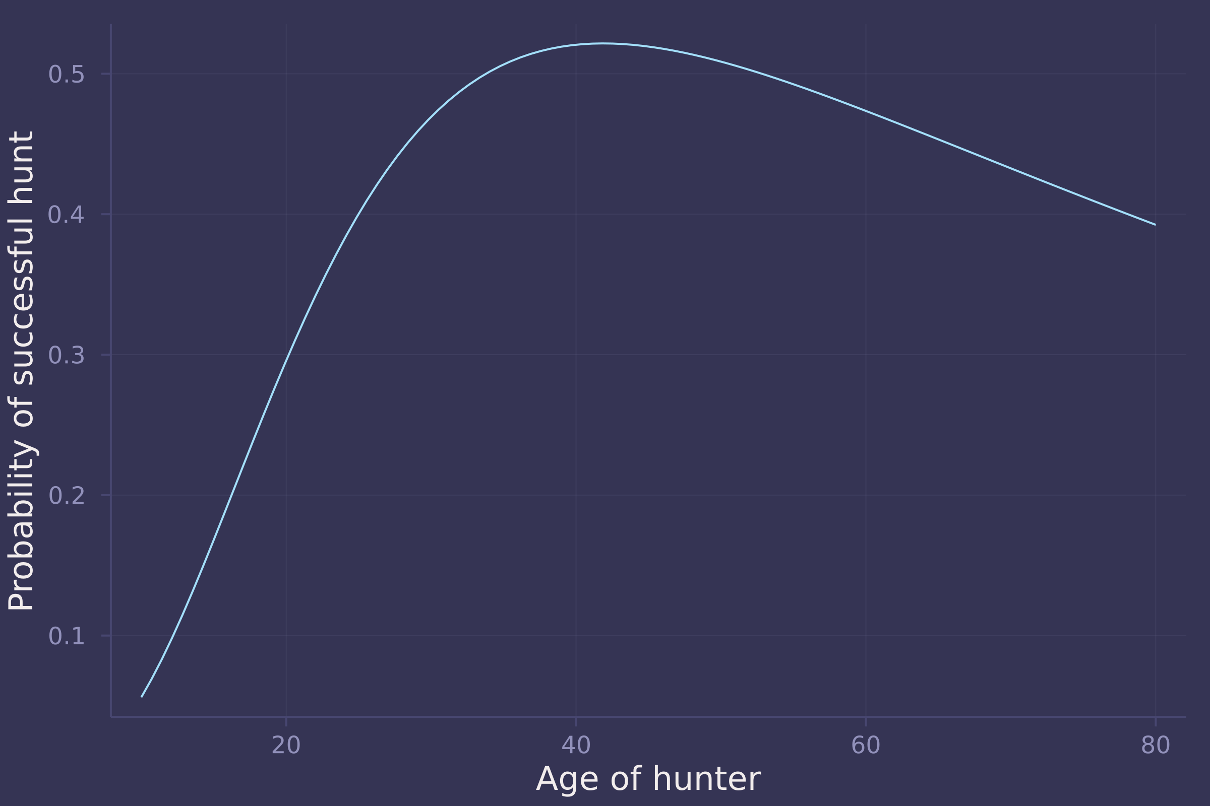
plot(age_seq .* maximum(trips.age), mean_prob_success, ylab="Probability of successful hunt", xlab="Age of hunter", legend=false)
@model function hunting2(s, a, hunter_id, n_hunters)
    σ ~ Exponential(1)
    τ ~ Exponential(1)
    η ~ Exponential(1)
    P ~ LKJ(2, η)
    v = Matrix(undef, n_hunters, 2)
    z ~ filldist(Normal(0, 1), 2, n_hunters)
    D = diagm([σ, τ])
    for i in 1:n_hunters
        v[i, :] = D * cholesky(P).L * vec(z[:, i])
    end
    α ~ Beta(4, 4)
    β ~ Normal(0, 0.5)
    γ ~ Normal(0, 0.5)
    δ ~ Exponential(0.5)
    ε = exp.(β .+ vec(v[1:n_hunters, 1]))
    ζ = exp.(γ .+ vec(v[1:n_hunters, 2]))
    p = α .* exp.(-ζ[hunter_id] .* a) .* ((1 .- exp.(-ε[hunter_id] .* a)) .^ δ)
    s .~ Bernoulli.(p)
end;

# reduce size of dataset for demonstration purposes!
trips2 = trips[1:111, :];

trips2.hunter_id = [findfirst(id .== unique(trips2.id)) for id in trips2.id];

model_hunting2 = hunting2(trips2.success, trips2.age ./ maximum(trips2.age), trips2.hunter_id, maximum(trips2.hunter_id));
post_hunting2 = sample(model_hunting2, NUTS(), 4000);

post_hunting2[["α", "β", "γ", "δ", "σ", "τ"]]
## Chains MCMC chain (4000×6×1 Array{Float64, 3}):
##
## Iterations        = 1001:1:5000
## Number of chains  = 1
## Samples per chain = 4000
## Wall duration     = 63.85 seconds
## Compute duration  = 63.85 seconds
## parameters        = σ, τ, α, β, γ, δ
## internals         =
##
## Summary Statistics
##   parameters      mean       std   naive_se      mcse         ess      rhat    ⋯
##       Symbol   Float64   Float64    Float64   Float64     Float64   Float64    ⋯
##
##            σ    0.8937    0.8794     0.0139    0.0133   3643.9991    0.9998    ⋯
##            τ    0.4947    0.4469     0.0071    0.0112   1647.0174    1.0003    ⋯
##            α    0.5722    0.1218     0.0019    0.0024   3251.8017    0.9998    ⋯
##            β    0.0744    0.4869     0.0077    0.0082   3560.4339    1.0006    ⋯
##            γ   -0.2992    0.3665     0.0058    0.0072   2742.6807    0.9998    ⋯
##            δ    0.3093    0.3012     0.0048    0.0054   3243.0843    0.9998    ⋯
##                                                                 1 column omitted
##
## Quantiles
##   parameters      2.5%     25.0%     50.0%     75.0%     97.5%
##       Symbol   Float64   Float64   Float64   Float64   Float64
##
##            σ    0.0202    0.2604    0.6226    1.2457    3.2864
##            τ    0.0167    0.1760    0.3842    0.6886    1.5920
##            α    0.3540    0.4824    0.5651    0.6600    0.8156
##            β   -0.9074   -0.2477    0.0736    0.3976    1.0232
##            γ   -1.0965   -0.5331   -0.2765   -0.0409    0.3427
##            δ    0.0063    0.0886    0.2202    0.4376    1.0983
Updated January 27, 2022 with Homework 1 and Homework 2 solutions
Updated February 10, 2022 with Homework 3 solutions
Updated February 24, 2022 with Homework 4 solutions
Updated March 10, 2022 with Homework 5 solutions
Updated March 24, 2022 with Homework 6 solutions
Updated April 7, 2022 with Homework 7 solutions
Updated April 21, 2022 with Homework 8 solutions
Updated May 5, 2022 with Homework 9 solutions