Kenya Population and Housing Census 2019

library(tidyverse)
library(rKenyaCensus)  # remotes::install_github("Shelmith-Kariuki/rKenyaCensus")
library(ggridges)
library(ggdark)

census <- rKenyaCensus::V3_T2.3 %>%
  rename_with(tolower) %>%
  filter(subcounty == "ALL") %>%
  select(county, age, total)

county_totals <- census %>%
  filter(age == "Total") %>%
  arrange(desc(total))

most_populous_counties <- county_totals %>%
  slice_max(total, n = 5) %>%
  pull(county)

most_populous_counties

census_ya <- census %>%
  filter(
    county %in% most_populous_counties,
    age %in% as.character(c(0:99), "100+")
  ) %>%
  mutate(
    age = as.numeric(recode(age, "100+" = "100")),
    is_young_adult = factor(ifelse((age > 17) & (age < 36), TRUE, FALSE)),
    county = fct_relevel(county, rev(most_populous_counties))
  ) 

census_ya %>%
  select(county, is_young_adult, total) %>%
  group_by(county) %>%
  mutate(county_total = sum(total)) %>%
  ungroup() %>%
  group_by(county, is_young_adult) %>%
  summarize(prop = sum(total / county_total)) %>%
  ungroup()

county_labels <- tribble(
  ~x, ~y, ~label,
  -3, 6.75, "Nairobi",
  -3, 4.93, "Kiambu",
  -3, 3.85, "Nakuru",
  -3, 2.65, "Kakamega",
  -3, 1.60, "Bungoma"
)

percent_labels <- tribble(
  ~x, ~y, ~label,
  27, 5.72, "43%",
  27, 4.27, "37%",
  27, 3.21, "32%",
  27, 2.13, "26%",
  27, 1.11, "27%"
)

ggplot(census_ya) +
  geom_density_ridges_gradient(aes(x = age, y = county, height = total, group = county, fill = is_young_adult), stat = "identity", scale = 2, color = "#f8f8f2") +
  geom_text(data = county_labels, aes(x, y, label = label), hjust = 1, family = "Inter-Medium", size = 5) +
  geom_text(data = percent_labels, aes(x, y, label = label), family = "Inter-Light", size = 4, alpha = 0.5) +
  scale_fill_manual(values = c("#282a36", "#44475a")) +
  scale_x_continuous(breaks = c(1, 18, 35, 100), labels = c(1, 18, 35, "100+")) + 
  expand_limits(x = c(-15, Inf)) +
  guides(fill = FALSE) +
  labs(
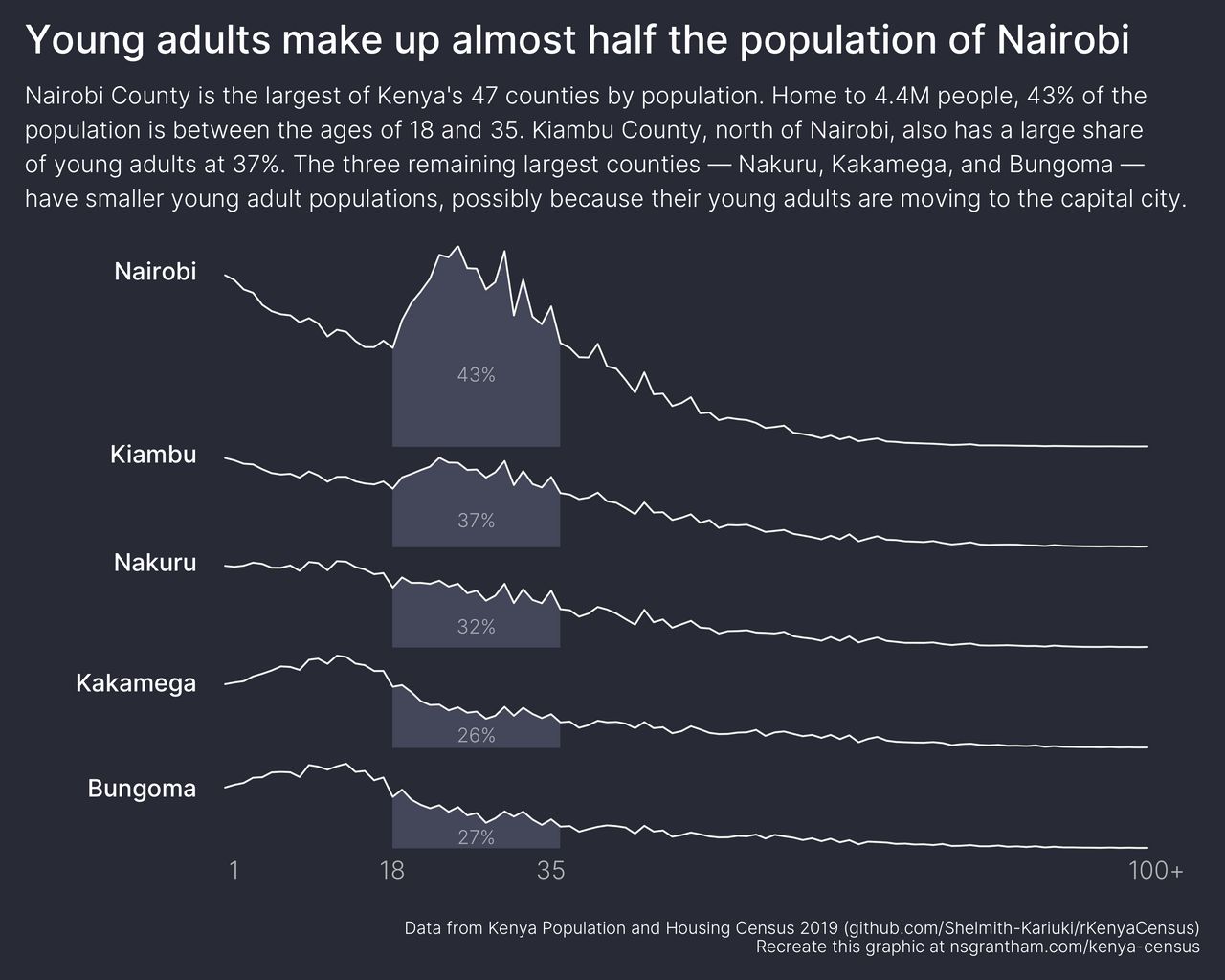
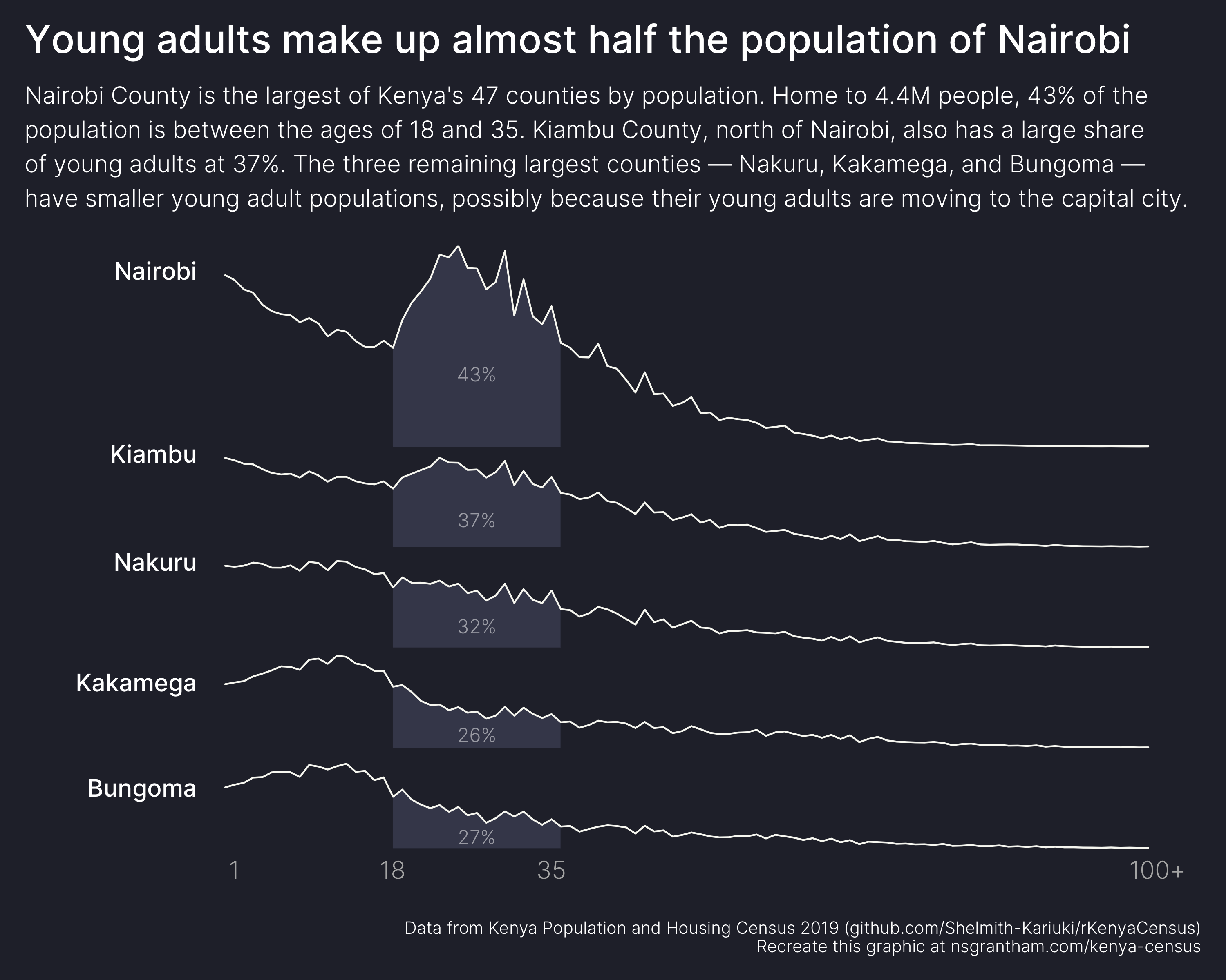
    title = "Young adults make up almost half the population of Nairobi",
    subtitle = "Nairobi County is the largest of Kenya's 47 counties by population. Home to 4.4M people, 43% of the\npopulation is between the ages of 18 and 35. Kiambu County, north of Nairobi, also has a large share\nof young adults at 37%. The three remaining largest counties — Nakuru, Kakamega, and Bungoma —\nhave smaller young adult populations, possibly because their young adults are moving to the capital city.",
    caption = "Data from Kenya Population and Housing Census 2019 (github.com/Shelmith-Kariuki/rKenyaCensus)\nRecreate this graphic at nsgrantham.com/kenya-census",
    x = NULL,
    y = NULL
  ) +
  dark_theme_minimal(base_family = "Inter-Light", base_size = 18) +
  theme(
    plot.background = element_rect(color = "#282a36", fill = "#282a36"),
    plot.title = element_text(family = "Inter-Medium", size = 23, margin = margin(0, 0, 0.7, 0, unit = "line")),
    plot.title.position = "plot",
    plot.subtitle = element_text(size = 14, lineheight = 1.2, margin = margin(0, 0, 1.2, 0, unit = "line")),
    plot.caption = element_text(size = 10),
    plot.margin = margin(1, 1, 1, 1, unit = "line"),
    panel.grid.major.y = element_blank(),
    panel.grid.major.x = element_blank(),
    panel.grid.minor.x = element_blank(),
    axis.text.y = element_blank(),
    axis.text.x = element_text(margin = margin(-2.5, 0, 1, 0, unit = "line"))
  )

ggsave("kenya-census.png", width = 10, height = 8)