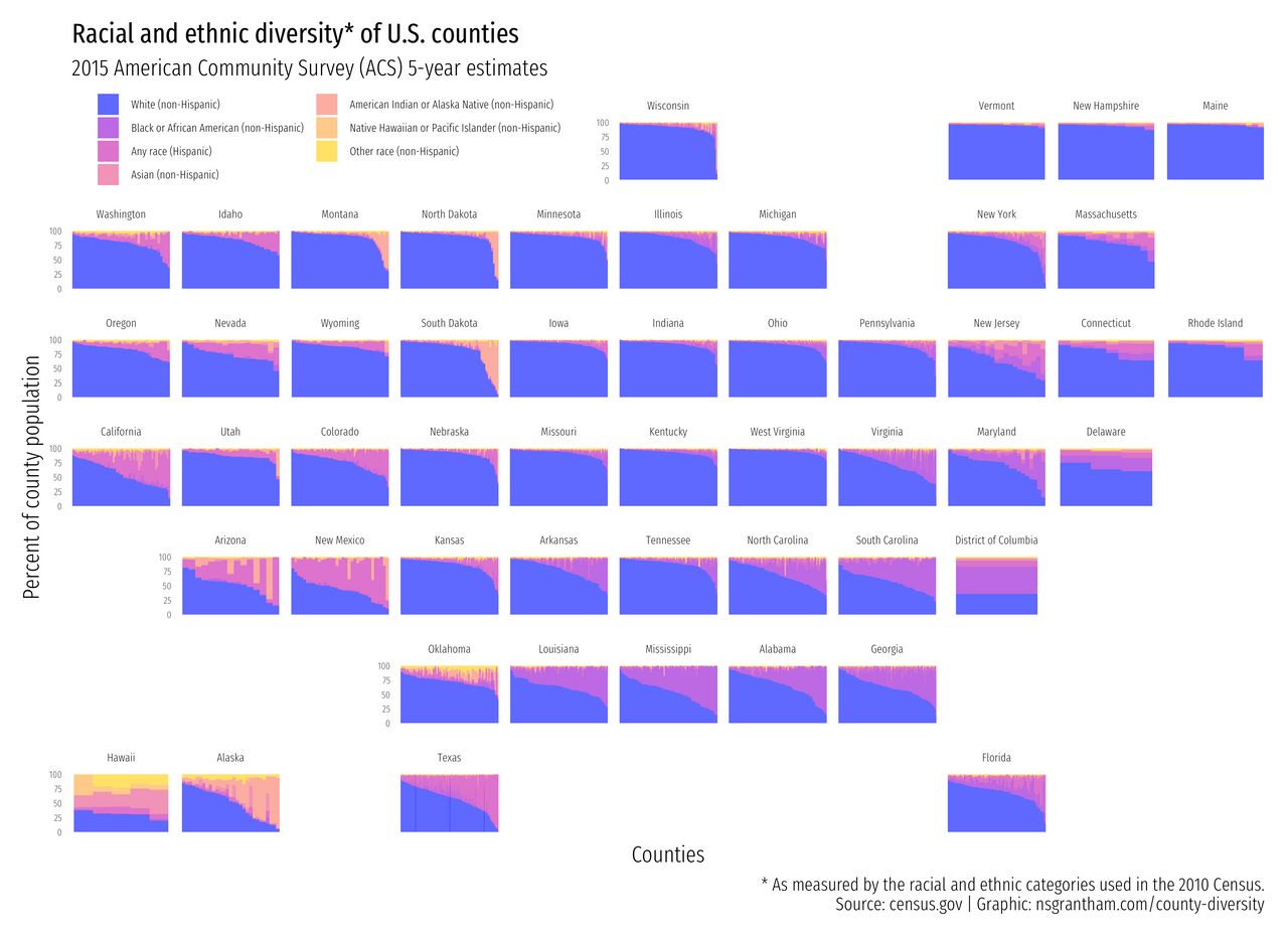
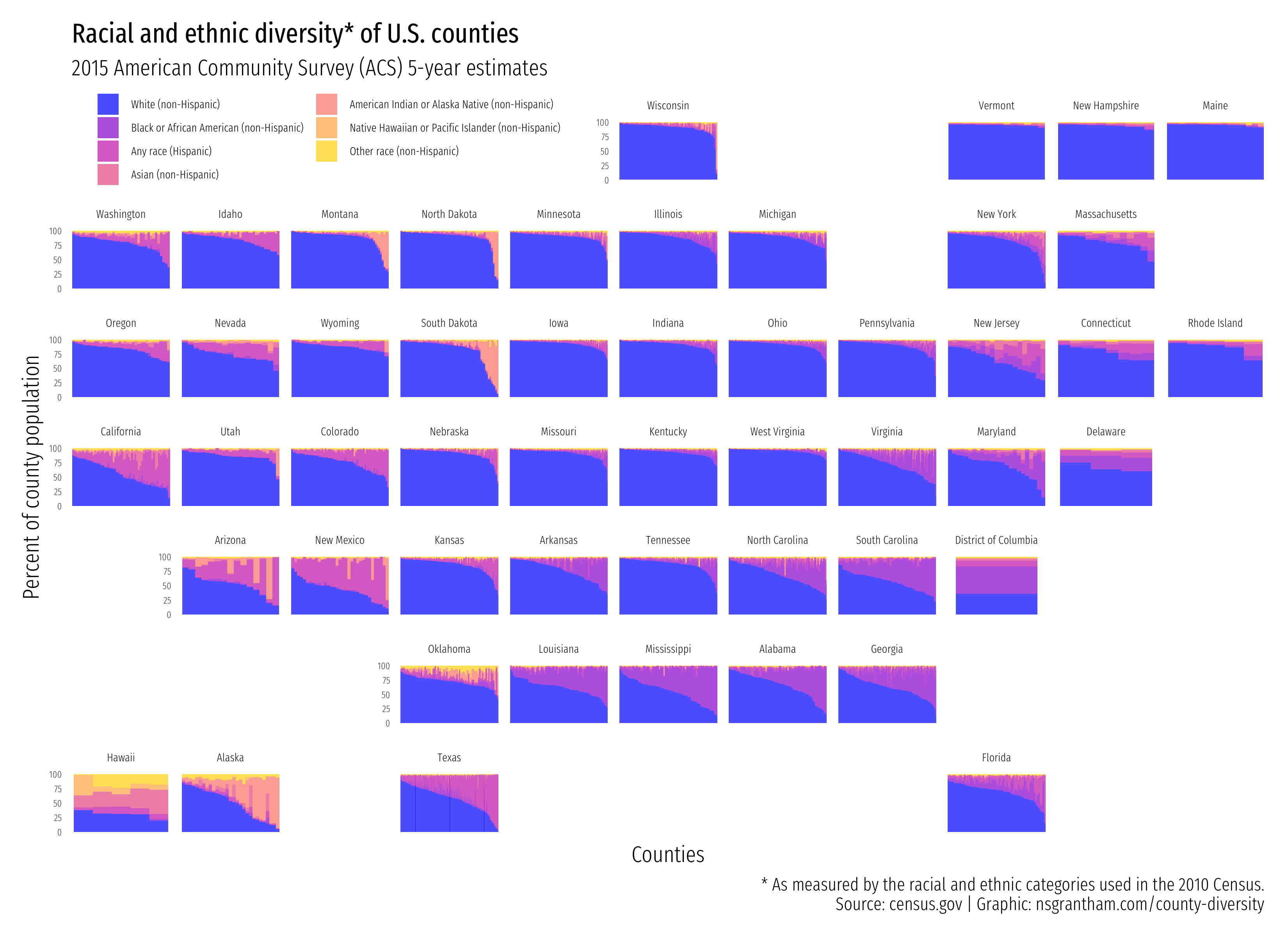
In this post we use American Community Survey (ACS) data from 2015 to examine the racial and ethnic diversity of counties in the United States.
library(tidyverse)
library(geofacet)

acs <- read_csv("https://raw.githubusercontent.com/rfordatascience/tidytuesday/master/data/2018/2018-04-30/week5_acs2015_county_data.csv") %>%
  select(CensusId, County, State, Hispanic, White, Black, Native, Asian, Pacific) %>%
  mutate(
    Other = 100 - Hispanic - White - Black - Native - Asian - Pacific,
    Other = replace(Other, Other < 0, 0),
    TotalPercent = Hispanic + White + Black + Native + Asian + Pacific + Other
  ) %>%
  mutate_at(vars(Hispanic, White, Black, Native, Asian, Pacific, Other), list(~ 100 * (. / TotalPercent))) %>%
  mutate(CensusId = fct_reorder(factor(CensusId), White, .desc = TRUE)) %>%
  gather(Race, PercentPop, Hispanic, White, Black, Native, Asian, Pacific, Other) %>%
  mutate(Race = factor(Race, levels = rev(c("White", "Black", "Hispanic", "Asian", "Native", "Pacific", "Other"))))

labels <- rev(c(
  "White (non-Hispanic)", "Black or African American (non-Hispanic)",
  "Any race (Hispanic)", "Asian (non-Hispanic)",
  "American Indian or Alaska Native (non-Hispanic)",
  "Native Hawaiian or Pacific Islander (non-Hispanic)",
  "Other race (non-Hispanic)"
))


ggplot(acs, aes(CensusId, PercentPop, fill = Race)) +
  geom_bar(stat = "identity", alpha = 0.7, width = 1) +
  facet_geo(~ State, grid = "us_state_grid1", scales = "free_x") +
  scale_fill_manual(labels = labels, values = c("#ffd700", "#ffb14e", "#fa8775", "#ea5f94", "#cd34b5", "#9d02d7", "#0000ff")) +
  labs(
    title = "Racial and ethnic diversity* of U.S. counties",
    subtitle = "2015 American Community Survey (ACS) 5-year estimates",
    x = "Counties",
    y = "Percent of county population",
    caption = paste(
      "* As measured by the racial and ethnic categories used in the 2010 Census.",
      "Source: census.gov | Graphic: nsgrantham.com/county-diversity",
      sep = "\n"
    )
  ) +
  guides(fill = guide_legend(ncol = 2, reverse = TRUE)) +
  theme_minimal(base_family = "Fira Sans Extra Condensed Light", base_size = 14) +
  theme(
    plot.title = element_text(family = "Fira Sans Extra Condensed"),
    plot.margin = unit(c(1, 1, 1, 1), "line"),
    legend.position = c(0.215, 0.965),
    legend.title = element_blank(),
    legend.text = element_text(size = 7),
    legend.key.size = unit(1, "line"),
    strip.text.x = element_text(size = 7),
    axis.text.y = element_text(size = 6),
    axis.text.x = element_blank(),
    panel.grid = element_blank()
  )

ggsave("county-diversity.png", width = 11, height = 8)